
1. Introduction
All graphs considered in this paper are simple, finite and undirected. In general we follow [1] and [16] for graph terminology and notations. Let \(G=(V,E)\) be a graph with vertex set \(V(G)\) and edge set \(E(G)\). For a vertex \(x \in V(G)\), the neighborhood of \(x\), denoted by \(\mathcal{N}(x)\), is the set of all vertices adjacent to \(x\). The degree of a vertex \(x\) is the cardinality of \(\mathcal{N}(x)\), and the minimum degree of \(G\) is denoted by \(\delta(G)\). A vertex of degree \(1\) is called a pendant vertex, whereas a universal vertex is one that is adjacent to every other vertex of the graph.
Graph coloring is a central topic in graph theory with a wide range of theoretical and practical applications. A particularly interesting variant, introduced by Chen et al. [3], is the coupon coloring of graphs, which models situations where each vertex must have access to all resources (colors) through its neighbors. Let \(G\) be a graph with no isolated vertices. A \(k\)-coupon coloring of \(G\) is an assignment of colors from \([k]=\{1,2,\ldots,k\}\) to the vertices of \(G\) such that the neighborhood of every vertex of \(G\) contains vertices of all colors from \([k]\). The maximum \(k\) for which a \(k\)-coupon coloring exists is called the coupon coloring number of \(G\), and is denoted by \(\chi_{c}(G)\) [3]. Clearly, \(\chi_{c}(G)\leq \delta(G)\) for any graph \(G\). In a \(k\)-coloring \(c\), a vertex \(v\) is considered to be a bad vertex if its neighborhood does not contain vertices of all colors from \([k]\) and it is clear that there are no bad vertices in a coupon coloring [15]. The notion of coupon coloring is closely related to graph domination. Let \(G = (V, E)\) be a graph without isolated vertices. \(D^{‘} \subseteq V\) is a total dominating set if every vertex of \(G\) is adjacent to at least one vertex in \(D^{‘}\). The coupon coloring number is also referred to as the total domatic number introduced in [12], which is the maximum number of disjoint total dominating sets. Total domatic number and coupon coloring have been extensively studied. The coupon coloring numbers of wheels, cycles, unicyclic and bicyclic graphs, complete graphs, and complete k-partite graphs were determined by Y Shi et al. in [15]. Additionally, coupon coloring has been examined in [14, 4] and [12]. The coupon coloring number of a few binary products, including the lexicographic and cartesian products is studied in [6, 13]. Also in [10] the authors have demonstrated that for every \(k \geq 3\), it is NP-complete to decide whether \(d_t(G) \geq k\), where \(G\) is split graph. Similarly, [10] shows that determining whether a bipartite planar graph has \(d_t(G) \geq 3\) is NP-complete.
Inflation is a unary graph operation that leaves the degree sequence unchanged while increasing the number of vertices and edges, and it has been examined in relation to total domination [7], double domination [11], as well as in various other studies [9, 8]. Cubic inflation was previously investigated in [2]. This paper studies coupon coloring in inflated graphs and introduces new inflation-based graph operations to examine their effect on coupon coloring.
2. Inflation of graphs
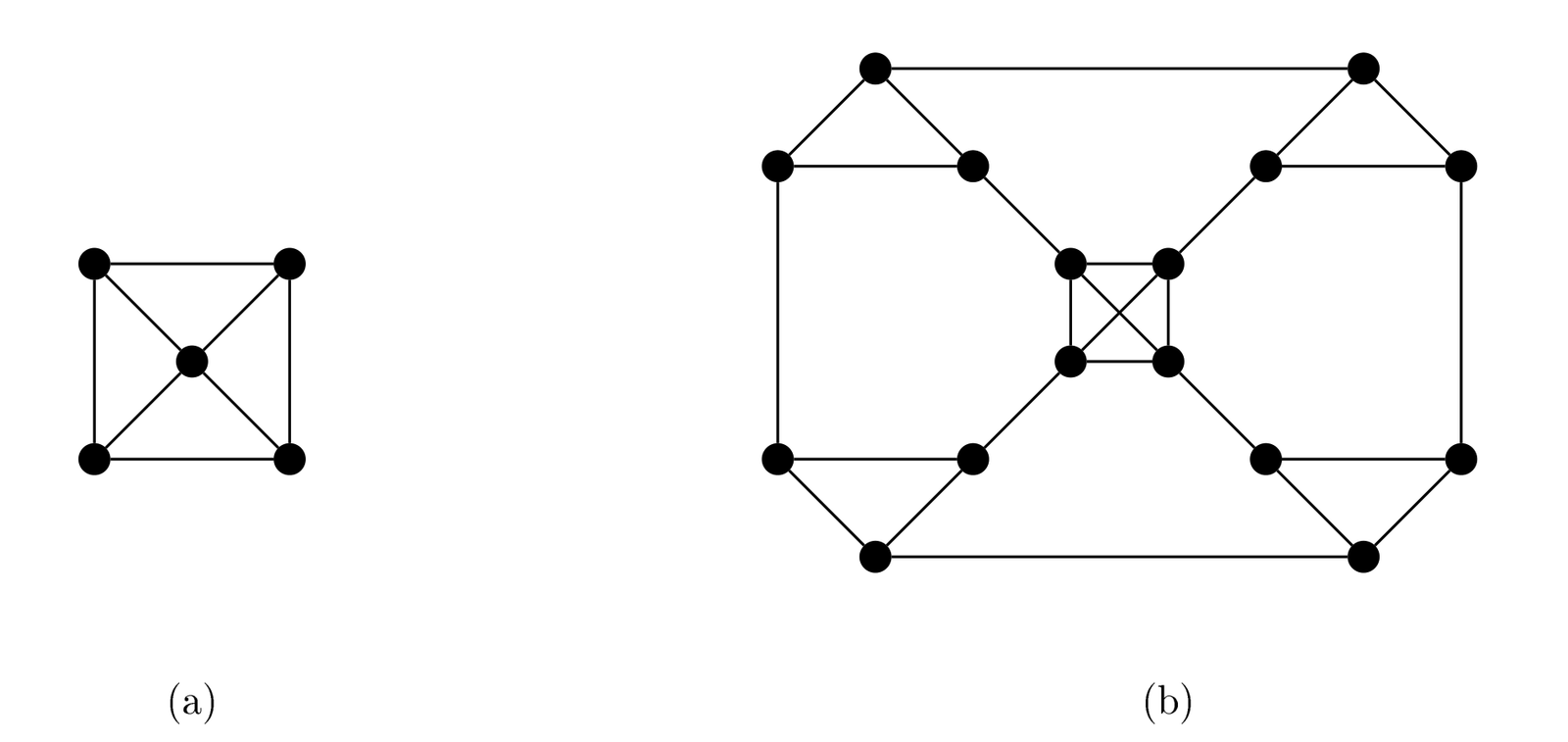
For the notation of inflated graphs, we follow [5]. The inflation \(G_I\) of a graph \(G\) is obtained by replacing each vertex \(v_i\) of degree \(d_G(v_i)\) with a clique \(K_i\) of size \(d_G(v_i)\). Each edge \(v_i v_j \in E(G)\) is replaced by an edge \(uv\) such that \(u \in K_i\) and \(v \in K_j\), and distinct edges of \(G\) are replaced by nonadjacent edges in \(G_I\). An immediate consequence of this definition is that \(n(G_I) = \sum\limits_{v_i \in V(G)} d_G(v_i) = 2m(G)\), \(\Delta(G_I) = \Delta(G),\) \(\delta(G_I) = \delta(G)\). Moreover, \(G_I\) can be seen as the line graph of the subdivision of \(G\). In \(G_I\), each vertex \(v_i\) of degree \(k\) in the original graph \(G\) is replaced by a clique of \(k\) vertices labeled \(v_i^1, v_i^2, \ldots, v_i^k\). Figure 1 illustrates Inflation of wheel.
Observation 2.1. Let \(G\) be any graph having a pendant vertex. After applying the inflation operation, the graph \(G_I\) also contains pendant vertex and hence \(\delta(G_I) = 1\). We know that \(\chi_{c}(G_I) \leq \delta(G_I)\). This implies that \(\chi_{c}(G_I) \leq 1\). Also \(G_I\) admits \(1\)-coupon coloring. Thus \(\chi_{c}(G_I)=1\)
Observation 2.2. Let \(G\) be a cycle graph on \(n\) vertices, then \((C_n)_I = C_{2n}\). Therefore,
Theorem 2.3. Let \(G=W_n\) be a wheel graph on \(n\) vertices. Then
Proof. Let \(G = W_n\) be a wheel graph on \(n\) vertices with vertex set \(v_1,v_2,\cdots,v_n\) and let \(v_1\) be the universal vertex. Here \(v_1\), having degree \(n-1\), is replaced by the set \(\{v_1^1, v_1^2, \ldots, v_1^{n-1}\}\), where each vertex \(v_1^i\) is adjacent to \(v_{i+1}^1\) in \(G_I\), corresponding to its neighbor \(v_{i+1}\) in \(G\). For each vertex \(v_i\) with \(i = 2, 3, \ldots, n\), the vertices \(v_i^2\) and \(v_i^3\) are connected in such a way that the sequence \(v_2^2 – v_2^3 – v_3^2 – v_3^3 – \cdots – v_n^2 – v_n^3 – v_2^2\) forms a cycle in \(G_I\), reflecting the cyclic structure among the vertices \(v_2, v_3, \ldots, v_n\) in \(G\). Since \(\delta(G_I)=3\), we have \(\chi_{c}(G_I)\leq 3\).
Case 1. \(n = 5\). For the case \(n = 5\), we have \(\delta(G_I) = 3\), so by the definition of coupon coloring, \(\chi_c(G_I) \leq 3\). Assume, for contradiction, that a valid 3-coupon coloring of \(G_I\) exists. Consider the vertex \(v_3^1\), which is adjacent to \(v_3^2\), \(v_3^3\), and \(v_1^2\). Without loss of generality, assign colors \(c(v_3^2) = 1\), \(c(v_3^3) = 2\), and \(c(v_1^2) = 3\). Now consider the vertex \(v_4^2\), whose neighbors are \(v_4^1\), \(v_4^3\), and \(v_3^3\). Since \(c(v_3^3) = 2\), and three colors must appear in the neighborhood, the possible colors for \(v_4^1\) are \(\{1, 3\}\).
Case 1.1. Suppose \(c(v_4^1) = 3\). This forces \(c(v_4^3) = 1\). Now, focusing on \(v_5^2\), which is adjacent to \(v_5^1\), \(v_5^3\), and \(v_4^3\), and since \(c(v_4^3) = 1\), we must have \(c(v_5^3) \in \{2, 3\}\).
Case 1.1.1. First, consider \(c(v_5^3) = 3\). This forces \(c(v_5^1) = 2\). Since \(v_5^1\) already has a neighbor colored 3, we assign \(c(v_5^2) = 1\). Otherwise if we assign \(c(v_5^2) =2\), then \(v_5^3\) will have two vertices in its neighborhood with same color \(2\), which makes \(v_5^3\) a bad vertex. Next,we consider the vertex \(v_5^3\), we get \(c(v_2^2) = 2\). Now we consider the neighboring vertices of the following vertices \(v_5^1, v_4^3,v_3^3,v_3^2,v_2^1,v_4^1\) and finally \(v_2^3\) in the order. This forces a cascade: \(c(v_2^2) = 3, \quad c(v_1^4) = 2,\quad c(v_4^2) = 2,\quad c(v_3^1) = 3,\quad c(v_2^3) = 1,\quad c(v_1^1) = 2,\quad c(v_1^3) = 3, \quad c(v_2^1)=3\). As a result, all vertices \(v_1^i\) for \(1 \leq i \leq 4\) become “bad” since their neighborhoods such as the vertices \(v_i^j\) where \(2 \le i \le 5\) and \(1 \le j \le 3\) lack the color \(1\).
Case 1.1.2. Let \(c(v_5^3) = 2\), then \(c(v_5^1) = 3\). Given that \(v_5^1\) has a neighbor colored 2, we must set \(c(v_5^2) = 1\), otherwise \(v_5^3\) will become the bad vertex. This again leads to: \(c(v_2^2) = 2,\quad c(v_1^4) = 3,\quad c(v_4^2) = 2,\quad c(v_3^1) = 3,\quad c(v_2^3) = 1,\quad c(v_1^1) = 3,\quad c(v_1^3) = 3, \quad c(v_2^1)=3\). Once again, all vertices \(v_1^i\) for \(1 \leq i \leq 4\) become bad since they lack the color \(1\) in its neighboring vertices which is \(v_i^j\) where \(2 \le i \le 5\) and \(1 \le j \le 3\).
Case 1.2. Suppose \(c(v_4^1) = 1\). Then, we must have \(c(v_4^3) = 3\). Now consider the vertex \(v_5^2\), which is adjacent to \(v_5^1\), \(v_5^3\), and \(v_4^3\). Since \(c(v_4^3) = 3\), the possible colors for \(v_5^3\) are 1 and 2.
Case 1.2.1. Assume \(c(v_5^3) = 2\). This forces \(c(v_5^1) = 1\). Since \(v_5^1\) already has a neighbor with color \(2\), we assign \(c(v_5^2) = 3\), otherwise if we assign \(c(v_5^2)=1\) this will force \(v_5^3\) to become a bad vertex. This leads to the following color assignments: \(c(v_2^2) = 2\) and \(c(v_1^4) = 1\). Also, \(c(v_4^2) = 2\), which implies \(c(v_1^3) = 1\). Considering the vertex \(v_3^3\), we get \(c(v_3^1) = 3\), and subsequently \(c(v_2^3) = 1\), which leads to \(c(v_1^1) = 3\), \(c(v_2^1)=3\). As a result, all vertices \(v_1^i\) for \(1 \leq i \leq 4\) become “bad” since their neighborhoods fail to contain the color \(2\).
Case 1.2.2. Alternatively, assume \(c(v_5^3) = 1\). Then \(c(v_5^1) = 2\). Since \(v_5^3\) has a neighbor with color \(2\), we get \(c(v_5^2) = 3\). This forces: \(c(v_2^2) = 1\) and \(c(v_1^4) = 2\). Also, \(c(v_4^2) = 2\), which implies \(c(v_1^3) = 1\). Considering \(v_3^3\), we get \(c(v_3^1) = 3\), and then \(c(v_2^3) = 1\). In this scenario, the vertex \(v_2^1\) becomes a bad vertex, since its neighborhood contain two vertices with same color \(1\) and hence all the required three colors are not present in the neighborhood.
In both cases, a contradiction arises, thereby showing that a valid 3-coupon coloring is not possible when \(n = 5\). To prove this we define \(C:V(G_I) \rightarrow [2]\) as follows. Let \(c(v_1^1)=c(v_1^2)=c(v_2^1)=c(v_3^1)=c(v_4^2)=c(v_4^3)=c(v_5^2)=c(v_5^3)=1\) and color all the other vertices with the color \(2\). This is indeed a coupon coloring. Thus \(\chi_{c}(G_I)=2\) when \(n=5\).
Case 2. \(n \neq 5\). Define a coloring function \(c : V(G_I) \rightarrow [3]\) as follows.
Case 2.1. \(n \equiv 0 \pmod{3}\). Assign \(c(v_1^{n-1}) = c(v_1^{n-2}) = c(v_{n-1}^1) = c(v_n^1) = 3\), \(c(v_{n-1}^2) = c(v_n^3) = 2\), and \(c(v_{n-1}^3) = c(v_n^2) = 1\). For \(1 \leq j \leq n – 3\), define:
Then, for \(2 \leq i \leq n – 2\) and \(1 \le j \le 3\) define \(c(v_i^j)=(i+j-3)\pmod{3}+1\).
Case 2.2. \(n \equiv 1 \pmod{3}\). For \(1 \leq j \leq n – 1\), define
For \(2 \leq i \leq n\) and \(1 \le j \le 3\) we define \(c(v_i^j)=(i+j-3)\pmod{3}+1\).
Case 2.3. \(n \equiv 2 \pmod{3}\) and \(n > 5\). Set \(c(v_1^{n-1}) = c(v_{n-1}^2) = 1\), \(c(v_1^{n-2}) = c(v_n^3) = 2\), and \(c(v_{n-1}^3) = c(v_n^2) = 3\). For \(1 \leq j \leq n – 3\):
For \(j \neq 1\) and \(2 \leq i \leq n\):
\(\square\)
Theorem 2.4. Let \(G=K_{m,n}\) be a complete bipartite graph on \(m+n\) vertices. Then \(\chi_{c}(G_{I})=min\{m,n\}\).
Proof. Let \(G = K_{m,n}\) be a complete bipartite graph with \(m + n\) vertices, and assume without loss of generality that \(m \leq n\). In \(G_I\), each vertex \(v_i\) of degree \(k\) is replaced by a clique of \(k\) vertices labeled \(v_i^1, v_i^2, \ldots, v_i^k\). The graph \(G_I\) has a vertex set \(V’ = V_1′ \cup V_2’\), where \(V_1′ = \{v_1^1, v_1^2, \ldots, v_1^n, v_2^1, v_2^2, \ldots, v_2^n, \ldots,\) \(v_m^1, v_m^2, \ldots, v_m^n\}\) and \(V_2′ = \{v_{m+1}^1, v_{m+1}^2, \ldots, v_{m+1}^m, v_{m+2}^1, v_{m+2}^2, \ldots,\) \(v_{m+2}^m, \ldots, v_{m+n}^1, v_{m+n}^2, \ldots, v_{m+n}^m\}\). Also each vertex \(v_i^j \in V_1’\) is connected to the vertex \(v_{m+j}^i \in V_2’\). Since every vertex in \(G_I\) has degree at least \(m\), we have \(\chi_c(G_I) \leq m\). We need to only show that \(\chi_c(G_I) \geq m\). Define \(c: V(G_I) \to [m]\) in the following way.
This ensures that each vertex sees all \(m\) colors in its neighborhood. Consider \(V_1^{‘}\), the replacement vertices of \(v_i \in V_1\) has the colors \(1,2, \cdots,m\) along with one more color from these \(m\) colors. So each vertex in \(V_1^{‘}\) will have \(m-1\) colors among the replacement vertices of \(v_i\) itself since the replacement vertices form a clique due to inflation. The only color that is not present in its neighborhood would be its own color. The vertex \(v_i^j \in V_1^{‘}\) is adjacent to \(v_{m+j}^{i} \in V_2^{‘}\). When \(i+j-1 \neq m\), \(c(v_i^j)=c(v_{m+j}^i)=i+j-1 \pmod{m}\). Similarly the case when \(i+j-1=m\). Hence the vertex \(v_i^j \in V_1^{‘}\) will have all \(m\) colors in its neighborhood. Similarly consider the vertices \(v_i^j \in V_2^{‘}\) where \(m+1 \le i \le m+n\) and \(1 \le j \le m\), each of these vertices will have all the colors among its neighboring vertices in \(V_2^{‘}\) which is nothing but the replacemnt vertices of \(v_i\) except its own color and this missing color will be present in the neighboring vertex that belongs to \(V_1^{‘}\). This ensures that the neighborhood of every vertex contains all \(m\) colors, satisfying the requirement for a valid \(m\)-coupon coloring. \(\square\)
3. \(\alpha\)-Operation
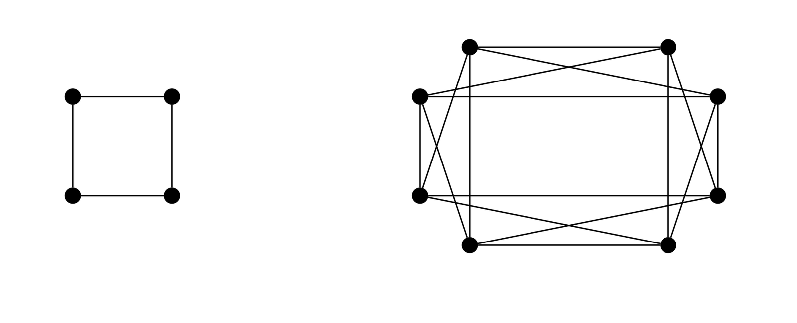
Definition 3.1. Let \(G\) be a graph of order \(n\) with no isolated vertices. Construct a new graph \(G_\alpha\) by replacing each vertex \(v_i \in V(G)\) of degree \(k\) with an independent set of \(k\) vertices, labelled \(v_i^1,v_i^2, \cdots ,v_i^k\). Whenever \(v_iv_l \in E(G)\), a complete join is made between the replacement set of \(v_i\) and the replacement set of \(v_l\). Order of \(G_\alpha\) is \(\sum\limits_{i=1}^{n} \deg(v_i)\). Figure 2 illustrates cycle of order \(4\) and \(\alpha\)-operation of cycle.
Theorem 3.2. Let \(G=P_n\) be a path on \(n\) vertices. Then
Proof. Let \(G = P_n\) be a path on \(n\) vertices with vertex set \(V(G) = \{v_1, v_2, \ldots, v_n\}\). Applying the alpha operation to \(G\), we obtain a new graph \(G_\alpha\), whose vertex set is \(V(G_\alpha) = \{v_1^1, v_2^1, v_2^2, \ldots, v_n^1\}\), where each original vertex \(v_i\) of degree \(k\) is replaced by \(k\) new vertices forming an independent set. In the case of a path, each internal vertex \(v_i\) (for \(2 \leq i \leq n-1\)) has degree 2 and is replaced by two vertices \(v_i^1\) and \(v_i^2\), while the endpoints \(v_1\) and \(v_n\) have degree 1 and are replaced by a single vertex \(v_1^1\) and \(v_n^1\), respectively. The resulting graph \(G_\alpha\) has minimum degree \(\delta(G_\alpha) = 2\), which implies that the coupon coloring number satisfies \(\chi_c(G_\alpha) \leq 2\).
Case 1. \(n=2\). When \(n = 2\), the path graph \(P_2\) consists of two vertices connected by a single edge. Applying the alpha operation to \(P_2\) does not change its structure, since each vertex has degree 1 and is replaced by a single vertex, preserving the original edge. As a result \((P_2)_\alpha\) is the same as \(P_2\). Therefore, the coupon coloring number remains unchanged, and we have \(\chi_c(G_\alpha) = 1\) when \(n = 2\).
Case 2. \(n \neq 2\). We define a 2-coloring \(c: V(G_\alpha) \rightarrow [2]\) as follows: assign color 1 to all \(v_i^1\) for \(1 \leq i \leq n-1\), assign color 2 to \(v_n^1\), and assign color 2 to all \(v_i^2\) for \(2 \leq i \leq n-1\). This coloring ensures that every vertex has neighbors receiving both colors, thereby satisfying the coupon coloring condition. \(\square\)
Theorem 3.3. Let \(G=C_n\) be a cycle on \(n\) vertices. Then
Proof. Let \(G = C_n\) be a cycle on \(n\) vertices. Since \(\delta(G_\alpha) = 4\), it follows that \(\chi_c(G_\alpha) \leq 4\).
Case 1. When \(n \equiv 0 \pmod{4}\). We define a coloring function \(c : V(G_\alpha) \rightarrow [4]\) as follows.
Case 1.1. If \(\left\lceil \frac{i}{2} \right\rceil\) is odd, then assign
Case 1.2. If \(\left\lceil \frac{i}{2} \right\rceil\) is even, then assign
Case 2. \(n \not\equiv 0\pmod{4}\). Consider the vertex \(v_2^1\), whose neighboring vertices are \(\{v_1^1, v_1^2, v_3^1, v_3^2\}\). Assume that \(v_1^1\) and \(v_1^2\) receive colors \(1\) and \(2\), respectively or vice versa. This implies that \(v_3^1\) and \(v_3^2\) receive colors \(3\) and \(4\), as they must differ from the colors of the other neighbors of \(v_2\). That is, if \(v_3^1\) receives color \(3\), then \(v_3^2\) must receive color \(4\), and vice versa. Continuing like this we get three cases.
Case 2.1. \(n \equiv 1\pmod{4}\).
Thus we get a contradiction since \(v_n^1,v_n^2\) will become the bad vertices. Hence, we have \(\chi_{c}(G_\alpha) \leq 3\). Define a coloring function \(c : V(G_\alpha) \rightarrow [3]\) as follows: assign \(c(v_n^1) = 1\) and \(c(v_n^2) = 3\). For each \(1 \leq i \leq n-1\), set \(c(v_i^2) = 2\).
Case 2.2. \(n \equiv 2\pmod{4}\).
From this we get \(v_n^1,v_n^2\) are bad vertices. Thus \(\chi_{c}(G_\alpha)\leq 3\). We define the following coloring \(c:V(G_\alpha)\rightarrow [3]\) as follows. Set \(c(v_{n-1}^1)=c(v_n^1)=1\) and \(c(v_{n-1}^2)=c(v_{n}^2)=3\). Now for \(1 \leq i \leq n-2\), we have \(c(v_i^2)=2\) . Also when \(j=1\) we have
Case 2.3. \(n \equiv 3\pmod{4}\).
This leads to a contradiction, as the final pair \(v_n^1, v_n^2\) ends up with conflicting color requirements, thereby becoming bad vertices. Thus \(\chi_{c}(G_\alpha)\leq 3\). We need to only prove that \(\chi_{c}(G_\alpha)\geq 3\). Define \(c:V(G_\alpha)\rightarrow [3]\) as follows.
The coloring \(c\) clearly satisfies the coupon coloring conditions. Thus, when \(n \not\equiv 0 \pmod{4}\), we conclude that \(\chi_{c}(G_\alpha) = 3\). \(\square\)
Theorem 3.4. Let \(G=K_{n}\) be a complete graph on \(n\) vertices. Then \(\chi_{c}(G_{\alpha})= \frac{n(n-1)}{2}\).
Proof. Let \(G=K_n\) be a complete graph on \(n\) vertices with vertex set \(v_1,v_2, \cdots, v_n\). Here \(\delta(G_\alpha)=(n-1)^2\) and the order of \(G_\alpha\) is \(n(n-1)\). Since by Lemma 4.4 and \(\frac{n(n-1)}{2} 0\) it follows that \(\chi_{c}(G_\alpha) \leq \frac{n(n-1)}{2}\). We can prove \(\chi_{c}(G_\alpha) \geq \frac{n(n-1)}{2}\) by defining a coloring \(c:V(G_\alpha) \rightarrow [\frac{n(n-1)}{2}]\) as follows. We have two cases.
Case 1. \(n\equiv 0\pmod{2}\). For all \(1 \leq j \leq n-1\) we have
Case 2. \(n\equiv 1\pmod{2}\). For \(i=\lceil \frac{n}{2} \rceil\) set \(c(v_i^j)=j+(n-1)(i-1)\) for \(1 \leq j \leq \lfloor \frac{n-1}{2} \rfloor\) and \(c(v_i^j)=j+ \lfloor \frac{n-1}{2} \rfloor(2i-n-2)\) for \(\lfloor \frac{n-1}{2} \rfloor +1 \leq j \leq n-1\). For all \(1 \leq j \leq n-1\) we have
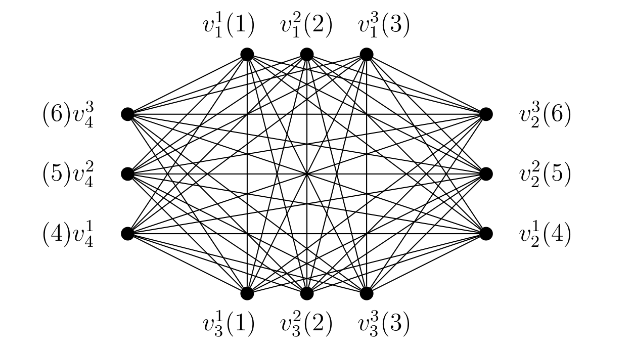
In Case \(1\), when \(n \equiv 0 \pmod{2}\), assign \(c(v_1^1)=1, c(v_1^2)=2,\cdots, c(v_1^{n-1})=n-1\). The replacement vertices of \(v_2\) receive the colors \(n,\ldots,2(n-1)\), and, in general, the replacement vertices of \(v_i\), \(2\le i\le \frac{n}{2}\), receive the colors \((i-1)(n-1)+1, \cdots, i(n-1)\). The replacement vertices of \(v_{\frac{n}{2}+1}\) are assigned the colors \(1,\cdots,n-1\), and the remaining replacement vertices are colored by continuing this pattern cyclically. Thus, each color appears exactly twice. Now let \(v_i\) be an arbitrary vertex. If \(1\le i\le \frac{n}{2}\), then the replacement vertices of \(v_j\), where \(\frac{n}{2}+1\le j\le n\), together contain all \(\frac{n(n-1)}{2}\) colors. Similarly, if \(\frac{n}{2}+1\le i\le n\), then the replacement vertices of \(v_j\), where \(1\le j\le \frac{n}{2}\), together contain all \(\frac{n(n-1)}{2}\) colors. Hence, the neighborhood of every arbitrary replacement vertex contains all \(\frac{n(n-1)}{2}\) colors. Moreover, each color appears exactly twice among the replacement vertices, completing the required coupon coloring. In Case 2 when \(n \equiv 1 \pmod{2}\) we have assigned \(c(v_1^1)=1,\; c(v_1^2)=2,\; \ldots,\; c(v_1^{n-1})=n-1\). For \(2 \le i \le \left\lceil \frac{n}{2}\right\rceil-1\), assign the replacement vertices of \(v_i\) the consecutive colors \((i-1)(n-1)+1,\; \ldots,\; i(n-1)\). The replacement vertices of \(v_{\left\lceil \frac{n}{2}\right\rceil}\) are assigned the colors \(\left(\left\lceil \frac{n}{2}\right\rceil-2\right)(n-1)+1,\; \ldots,\; \frac{n(n-1)}{2},\; 1,\; \ldots,\; \frac{n-1}{2}\). For \(\left\lceil \frac{n}{2}\right\rceil+1 \le i \le n\), the color assignment continues cyclically, with the replacement vertices of \(v_n\) receiving the colors \(\frac{(n-1)(n-2)}{2}+1,\; \ldots,\; \frac{n(n-1)}{2}\). Consequently, the neighborhood of every replacement vertex contains all \(\frac{n(n-1)}{2}\) colors. Moreover, each color appears exactly twice among the replacement vertices, completing the required coupon coloring. Thus \(\chi_{c}(G_{\alpha})= \frac{n(n-1)}{2}\). \(\square\)
Figure 3 illustrates coupon coloring of \(K_{4_\alpha}\).
Observation 3.5. Let \(G=K_{1,n}\) be a star graph on \(n+1\) vertices. Then \(\chi_{c}(G_\alpha)=n\).
Proof. Let \(G=K_{1,n}\) be a star graph on \(n+1\) vertices with vertex set \(\{v_1,v_2,\cdots,v_{n+1}\}\), where \(v_1\) is the universal vertex. \((K_{1,n})_\alpha\) is the graph \(K_{n,n}\). Thus \(\chi_{c}(K_{1,n})_\alpha=n\). \(\square\)
Theorem 3.6. Let \(G=S_{r,t}\) be a double star graph on \(r+t+2\) vertices. Then \(\chi_{c}(G_\alpha)=min \{r,t\}+1\).
Proof. Let \(G = S_{r,t}\) denote a double star graph with \(r+t+2\) vertices and vertex set \(V(G)=\{x,w,u_1,u_2, \cdots, u_r, v_1,v_2,\ldots,v_t\}\). The vertices \(x\) and \(w\) are adjacent. The set \(\{u_1,u_2,\ldots,u_r\}\) consists of leaves adjacent to \(x\), forming a star centered at \(x\), while \(\{v_1,v_2,\ldots,v_t\}\) consists of leaves adjacent to \(w\), forming a star centered at \(w\). Under the \(\alpha\)-operation, every vertex \(u_i\) of degree \(1\) is replaced by a single vertex denoted \(u_i^1\), and likewise for each vertex \(v_i\). The vertices \(x\) and \(w\), having degrees \(r+1\) and \(t+1\), respectively, are replaced by independent vertices labeled \(x^1, x^2, \ldots, x^{r+1}\) and \(w^1, w^2, \ldots, w^{t+1}\), respectively. Without loss of generality assume that \(r \leq t\). Since \(\delta(G_\alpha)=min \{r,t\}+1\), we have \(\chi_{c}(G_\alpha) \leq r+1\). We define \(c:V(G_\alpha)\rightarrow [r+1]\) as follows. Set \(c(w^i)=c(x^i)=i\) for all \(1 \leq i \leq r+1\). Remaining vertices can be colored using any color from \(1,2, \cdots,r\). Consider the replacement vertices of leaves in \(G\). In the case of \(u_i^1\) where \(1 \le i \le r\), these vertices are adjacent to \(x^h\), where \(1 \le h \le r+1\) which contains all the \(r+1\) colors. Similarly in the case of \(v_j^1\), where \(1 \le j \le t\), these vertices are adjacent to \(w^g\), where \(1 \le g \le t+1\). The vertices \(x^h\), where \(1 \le h \le r+1\) are adjacent to \(w^g\), where \(1 \le g \le t+1\). Hence these vertices will also have \(r+1\) colors in its neighborhood. \(\square\)
Observation 3.7. [15] Let \(G = (X,Y)\) be a complete bipartite graph with \(|X|=n_1\), \(|Y|=n_2\) and \(n_1 \leq n_2\). By the definition of the coupon coloring number, we can easily obtain that \(\chi_c(G) = n_1\).
Theorem 3.8. Let \(G=K_{m,n}\) be a complete bipartite graph on \(m+n\) vertices. Then \(\chi_{c}(G_\alpha)=mn\).
Proof. Let \(G=K_{m,n}\) be a complete bipartite graph on \(m+n\) vertices. Applying the alpha operation to the complete bipartite graph \(K_{m,n}\) results in the graph \(K_{mn,mn}\). From Observation 3.7 we get \(\chi_{c}(G_\alpha)=mn\). \(\square\)
4. \(\beta\)-Operation
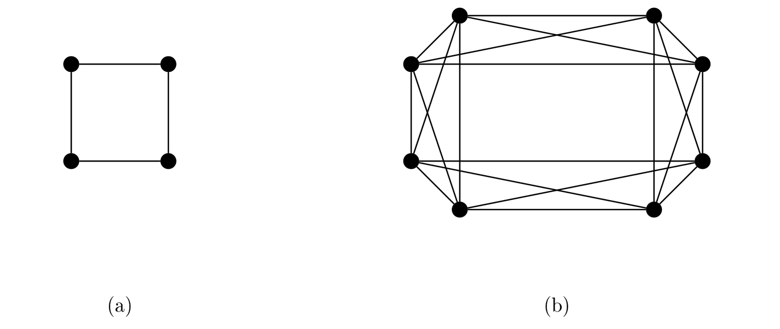
Definition 4.1. Let \(G\) be a graph of order \(n\) with no isolated vertices. Construct a new graph \(G_\beta\) by replacing each vertex \(v_i \in V(G)\) of degree \(k\) with a Path \(P_{v_i}\) on \(k\) vertices, labeled \(v_i^1, v_i^2, \ldots, v_i^k\). Whenever \(v_iv_j \in E(G)\), complete join is made between the vertices of \(P_{v_i}\) and \(P_{v_j}\). Order of \(G_\beta\) is \(\sum\limits_{i=1}^{n} \deg(v_i)\). Figure 4 illustrates cycle of order \(4\) and \(\beta\)-operation of cycle.
Theorem 4.2. Let \(G=P_n\) be a path on \(n\) vertices. Then
Proof. Let \(G=P_n\) be a path on \(n\) vertices.
Case 1. \(n=2\). When \(n=2\), \(P_{2_\beta}=P_2\).
Case 2. \(n \neq 2\). We have \(\chi_{c}({G_\beta}) \leq 2\). Define the following coloring \(c:V(G_\beta)\rightarrow [2]\) as follows. Set \(c(v_1^1)=1\) and \(c(v_n^1)=2\). For \(2 \leq i \leq n-1\) and \(j=1,2\), we have
\(c\) can be easily verified to be a coupon coloring. \(\square\)
Theorem 4.3. Let \(G=C_n\) be a cycle on \(n\) vertices. Then
Proof. Let \(G=C_n\) be a cycle on \(n\) vertices with vertex set \(v_1,v_2, \cdots, v_n\). Let \(v_1^1,v_1^2,v_2^1,v_2^2,\\\cdots,v_n^1,v_n^2\) be the vertices of \(G_\beta\) after applying \(\beta\) operation. We have \(\chi_{c}(G_\beta) \leq 5\). Suppose there exists a \(5\)-coupon coloring \(c:V(G_\beta)\rightarrow [5]\). Consider the vertex \(v_1^1\), the neighboring vertices are \(v_1^2,v_2^1,v_2^2,v_n^1,v_n^2\). Without loss of generality, assume that \(c(v_1^2)=1,c(v_2^1)=2,c(v_2^2)=3,c(v_n^1)=4,c(v_n^2)=5\). Now consider \(v_1^2\), we get \(c(v_1^1)=1\) which makes \(v_2^1\) the bad vertex. Thus \(\chi_{c}(G_\beta) \leq 4\).
Case 1. \(n \equiv 0\pmod{4}\). Define \(c:V(G_\beta)\rightarrow [4]\) as follows.
It can be readily verified that \(c\) is a coupon coloring.
Case 2. \(n \not\equiv 0\pmod{4}\). Consider the vertex \(v_1^1\), the neighboring vertices are \(v_1^2,v_2^1,v_2^2,v_n^1,\\ v_n^2\). Without loss of generality, assume that \(c(v_1^2)=1,c(v_2^1)=2,c(v_2^2)=3,c(v_n^1)=4\). Consider the vertex \(v_1^2\) we have two cases. Either \(c(v_1^1)=1\) or \(c(v_n^2)=1\).
Case 2.1. \(c(v_1^1)=1\). Examining the vertex \(v_2^1\) forces \(c(v_3^1)\) to be either \(2\) or \(4\). Assume that \(c(v_3^1)=2\). This implies that \(c(v_3^2)=4\), which leads to a contradiction, since the neighborhood of \(v_2^2\) does not contain the color \(3\). Similarly when \(c(v_3^1)=4\) implies \(c(v_3^2)=2\) and this also leads to contradiction since \(v_2^2\) become the bad vertex.
Case 2.2. \(c(v_n^2)=1\). Consider the vertices \(v_2^2\) and \(v_2^1\). Their neighborhoods must contain the colors \(2,3,\) and \(4\). We get three cases.
Case 2.2.1. \(c(v_1^1)=2\). Then we get either \(c(v_3^1)=4\) or \(c(v_3^2)=4\). if \(c(v_3^1)=4\), this implies \(c(v_3^2)=3\) and vice versa. In both these cases when we consider the vertices \(v_3^1\) and \(v_3^2\) we get \(c(v_4^1),c(v_4^2) \in \{1,4\}\). If \(c(v_4^1)=1\), then \(c(v_4^2)=4\) or viceversa. Hence for \(1 \le i \le n-1\) we get
Now \(n \equiv 1 \pmod{4}\) then \(v_n^1\) and \(v_n^2\) doesnot contain the color \(3\) in ite neighborhood, hence we get a contradiction. When \(n \equiv 2 \pmod{4}\) \(v_n^1\) and \(v_n^2\) doesnot contain the color \(3\) and \(4\) in ite neighborhood and when \(n \equiv 3 \pmod{4}\), \(v_n^1\) and \(v_n^2\) doesnot contain the color \(4\) in ite neighborhood, hence this also leads to contradiction.
Case 2.2.2. \(c(v_1^1)=3\). Then we get either \(c(v_3^1)=4\) or \(c(v_3^2)=4\). If \(c(v_3^1)=4\), this implies \(c(v_3^2)=2\) and vice versa. In both these cases when we consider the vertices \(v_3^1\) and \(v_3^2\) we get \(c(v_4^1),c(v_4^2) \in \{1,4\}\). If \(c(v_4^1)=1\), then \(c(v_4^2)=4\) or viceversa. Hence for \(1 \le i \le n-1\) we get
Now \(n \equiv 1 \pmod{4}\) then \(v_n^1\) and \(v_n^2\) doesnot contain the color \(2\) in ite neighborhood, hence we get a contradiction. When \(n \equiv 2 \pmod{4}\) \(v_n^1\) and \(v_n^2\) doesnot contain the color \(2\) and \(4\) in ite neighborhood and when \(n \equiv 3 \pmod{4}\), \(v_n^1\) and \(v_n^2\) doesnot contain the color \(4\) in ite neighborhood, hence this also leads to contradiction.
Case 2.2.3. \(c(v_1^1)=4\). Then we get either \(c(v_3^1)=2\) or \(c(v_3^2)=2\) if \(c(v_3^1)=2\), this implies \(c(v_3^2)=4\) and vice versa. In both these cases when we consider the vertices \(v_3^1\) and \(v_3^2\) we get \(c(v_4^1),c(v_4^2) \in \{1,4\}\). If \(c(v_4^1)=1\), then \(c(v_4^2)=4\) or viceversa. Hence for \(1 \le i \le n-1\) we get
Now \(n \equiv 1,2 \pmod{4}\) then \(v_n^1\) and \(v_n^2\) doesnot contain the colors \(2\) and \(3\) in its neighborhood, hence we get a contradiction and when \(n \equiv 3 \pmod{4}\), \(v_{n-1}^1\) and \(v_{n-1}^2\) doesnot contain the colors \(2\) and \(3\) in its neighborhood, hence this also leads to contradiction. Thus \(\chi_{c}(G_\beta) \leq 3\). Define \(c:V(G_\beta) \rightarrow [3]\) as follows.
Case 1. \(n \equiv 1 \pmod{4}\). Assign \(c(v_n^1) = 1\) and \(c(v_n^2) = 3\). For each \(1 \leq i \leq n-1\), set \(c(v_i^2) = 2\).
Case 2. \(n \equiv 2,3 \pmod{4}\).
In both cases if we consider an arbitary vertex \(v_i^j\), where \(2 \le i \le n-1\) and \(j=1,2\), the vertices \(v_{i-1}^j\) and \(v_{i+1}^j\) where \(j=1,2\) will contain all the required three colors. Hence all three colors will be present in the neighborhood of \(v_i^j\). Similarly for \(v_1^j\) and \(v_n^j\), where \(j=1,2\). Thus \(\chi_{c}(G_\beta)=3\) when \(n \not\equiv 0 \pmod{4}\). \(\square\)
Lemma 4.4. In coupon coloring each color should appear atleast twice.
Proof. Let \(G\) be a graph and for \(G\) to satisfy coupon coloring, each vertex should have all the colors in its neighboring vertices. If a color appears on exactly one vertex \(u\), then \(u\) itself cannot see that color in \(\mathcal{N}(u)\), so the coloring cannot be a coupon coloring. Similarly for all vertices. Thus each color should appear atleast twice to satisfy the coupon coloring condition. \(\square\)
Theorem 4.5. Let \(G=K_{n}\) be a complete graph on \(n\) vertices. Then \(\chi_{c}(G_{\beta})= \frac{n(n-1)}{2}\).
Proof. Let \(G=K_n\) be a complete graph on \(n\) vertices with vertex set \(v_1,v_2, \cdots, v_n\). Here \(\delta(G_\beta)=(n-1)^2+1\) and the order of \(G_\beta\) is \(n(n-1)\). Since by Lemma 4.4 and \(\frac{n(n-1)}{2} 0\) it follows that \(\chi_{c}(G_\beta) \leq \frac{n(n-1)}{2}\). We can prove \(\chi_{c}(G_\beta) \geq \frac{n(n-1)}{2}\) by defining a coloring \(c:V(G_\beta) \rightarrow [\frac{n(n-1)}{2}]\) as follows. We have two cases.
Case 1. \(n\equiv 0\pmod{2}\). For all \(1 \leq j \leq n-1\) we have
Case 2. \(n\equiv 1\pmod{2}\). For \(i=\lceil \frac{n}{2} \rceil\) set \(c(v_i^j)=j+(n-1)(i-1)\) for \(1 \leq j \leq \lfloor \frac{n-1}{2} \rfloor\) and \(c(v_i^j)=j+ \lfloor \frac{n-1}{2} \rfloor(2i-n-2)\) for \(\lfloor \frac{n-1}{2} \rfloor +1 \leq j \leq n-1\). For all \(1 \leq j \leq n-1\) we have
In Case \(1\), when \(n \equiv 0 \pmod{2}\), assign \(c(v_1^1)=1,\; c(v_1^2)=2,\; \ldots,\; c(v_1^{n-1})=n-1\). The replacement vertices of \(v_2\) receive the colors \(n,\ldots,2(n-1)\), and, in general, the replacement vertices of \(v_i\), \(2\le i\le \frac{n}{2}\), receive the colors \((i-1)(n-1)+1,\; \ldots,\; i(n-1)\). The replacement vertices of \(v_{\frac{n}{2}+1}\) are assigned the colors \(1,\ldots,n-1\), and the remaining replacement vertices are colored by continuing this pattern cyclically. Thus, each color appears exactly twice. Now let \(v_i\) be an arbitrary vertex. If \(1\le i\le \frac{n}{2}\), then the replacement vertices of \(v_j\), where \(\frac{n}{2}+1\le j\le n\), together contain all \(\frac{n(n-1)}{2}\) colors. Similarly, if \(\frac{n}{2}+1\le i\le n\), then the replacement vertices of \(v_j\), where \(1\le j\le \frac{n}{2}\), together contain all \(\frac{n(n-1)}{2}\) colors. Hence, the neighborhood of every arbitrary replacement vertex contains all \(\frac{n(n-1)}{2}\) colors. Moreover, each color appears exactly twice among the replacement vertices, completing the required coupon coloring. In Case 2 when \(n \equiv 1 \pmod{2}\) we have assigned \(c(v_1^1)=1,\; c(v_1^2)=2,\; \ldots,\; c(v_1^{n-1})=n-1\). For \(2 \le i \le \left\lceil \frac{n}{2}\right\rceil-1\), assign the replacement vertices of \(v_i\) the consecutive colors \((i-1)(n-1)+1,\; \ldots,\; i(n-1)\). The replacement vertices of \(v_{\left\lceil \frac{n}{2}\right\rceil}\) are assigned the colors \(\left(\left\lceil \frac{n}{2}\right\rceil-2\right)(n-1)+1,\; \ldots,\; \frac{n(n-1)}{2},\; 1,\; \ldots,\; \frac{n-1}{2}\). For \(\left\lceil \frac{n}{2}\right\rceil+1 \le i \le n\), the color assignment continues cyclically, with the replacement vertices of \(v_n\) receiving the colors \(\frac{(n-1)(n-2)}{2}+1,\; \ldots,\; \frac{n(n-1)}{2}\). Consequently, the neighborhood of every replacement vertex contains all \(\frac{n(n-1)}{2}\) colors. Moreover, each color appears exactly twice among the replacement vertices, completing the required coupon coloring. Thus \(\chi_{c}(G_{\beta})= \frac{n(n-1)}{2}\). \(\square\)
Theorem 4.6. Let \(G=K_{1,n}\) be a star graph on \(n+1\) vertices. Then \(\chi_{c}(G_\beta)=n\).
Proof. Let \(G = K_{1,n}\) be a star graph on \(n+1\) vertices, where \(v_1\) is the universal vertex and \(v_2, v_3, \ldots, v_{n+1}\) are the pendant vertices. We have \(\chi_{c}(G_\beta) \leq n\), since \(\delta(G_\beta)=n\). Define a coloring \(c : V(G_\beta) \rightarrow [n]\) as follows: \(c(v_1^j)=j\) where \(1 \le j \le n\), and \(c(v_i^1)=i-1\) where \(2 \le i \le n+1\). Then \(\chi_{c}(G_\beta)=n\). \(\square\)
Theorem 4.7. Let \(G=S_{r,t}\) be a double star graph on \(r+t+2\) vertices. Then \(\chi_{c}(G_\beta)=min \{r,t\}+1\).
Proof. Let \(G = S_{r,t}\) be a double star graph with \(r+t+2\) vertices and vertex set \(V(G)=\{x,w,u_1,u_2,\) \(\cdots, u_r, v_1,v_2,\ldots,v_t\}\). The vertices \(x\) and \(w\) are adjacent. The set \(\{u_1,u_2,\ldots,u_r\}\) consists of leaves adjacent to \(x\), forming a star centered at \(x\), while \(\{v_1,v_2,\ldots,v_t\}\) consists of leaves adjacent to \(w\), forming a star centered at \(w\). Under the \(\beta\)-operation, every vertex \(u_i\) of degree \(1\) is replaced by a single vertex denoted \(u_i^1\), and likewise for each vertex \(v_i\). The vertices \(x\) and \(w\), having degrees \(r+1\) and \(t+1\), respectively, are replaced by paths on \(r+1\) and \(t+1\) vertices labeled \(x^1, x^2, \ldots, x^{r+1}\) and \(w^1, w^2, \ldots, w^{t+1}\), respectively. Without loss of generality, assume that \(r \leq t\). Since \(\delta(G_\beta)=min \{r,t\}+1\), we have \(\chi_{c}(G_\beta) \leq r+1\). We define \(c:V(G_\beta)\rightarrow [r+1]\) as follows. Similar to Theorem 3.6 we set \(c(w^i)=c(x^i)=i\) for all \(1 \leq i \leq r+1\). Remaining vertices can be colored using any color from \(1,2, \cdots,r\). In the case of \(u_i^1\) where \(1 \le i \le r\), these vertices are adjacent to \(x^h\), where \(1 \le h \le r+1\) which contains all the \(r+1\) colors. Similarly in the case of \(v_j^1\), where \(1 \le j \le t\), these vertices are adjacent to \(w^g\), where \(1 \le g \le t+1\). The vertices \(x^h\), where \(1 \le h \le r+1\) are adjacent to \(w^g\), where \(1 \le g \le t+1\). Hence these vertices will also have \(r+1\) colors in its neighborhood. \(\square\)
Theorem 4.8. Let \(G=K_{m,n}\) be a complete bipartite graph on \(m+n\) vertices. Then \(\chi_{c}(G_\beta)=mn\).
Proof. Let \(G=K_{m,n}\) be a complete bipartite graph on \(m+n\) vertices with vertex set \(u_1,u_2,\cdots,u_m\) on one partition and \(v_1,v_2,\cdots,v_n\) on another partition. We have \(\chi_{c}(G_\beta) \leq mn+1\). Assume there exists an \(mn+1\)-coupon coloring, \(c:V(G_\beta) \rightarrow [mn+1]\). Now consider the vertex \(u_1^1\), the neighboring vertices are \(u_1^2\) and \(v_i^k\) for all \(1 \leq i \leq m\) and \(1 \leq k \leq n\). Without loss of generality, assume that \(c(v_1^1)=1, c(v_1^2)=2, c(v_1^3)=3, \cdots, c(v_1^m)=m, c(v_2^1)=m+1 \cdots, c(v_n^m)=mn\). We get \(c(v_i^j)=mi+j-m\). Hence \(c(u_1^2)=mn+1\). Now consider the vertex \(v_1^1\), the neighboring vertices are \(v_1^2\), which has color \(2\) and \(u_i^k\) for all \(1 \leq i \leq m\) in which \(u_1^2\) has color \(mn+1\). Without loss of generality, assume that \(c(u_1^1)=1, c(u_1^3)=3, \cdots, c(u_1^n)=n, c(u_2^1)=n+1, \cdots, c(u_m^n)=mn\). We get \(c(u_i^j)=ni+j-n\) for all \(i \neq 1\) and \(j \neq 2\). Two of the neighboring vertices of \(v_1^2\) have same color \(1\) and remaining there are \(mn-1\) neighboring vertices. We need to give \(mn\) colors to them and this is a contradiction since the vertex \(v_1^2\) will become a bad vertex. Consequently, \(\chi_c(G_\beta) \le mn\). Define a coloring \(c : V(G_\beta) \to [mn]\) by assigning \(c(u_i^j)=ni+j-n \quad \text{and} \quad c(v_i^j)=mi+j-m\). Since this assignment yields a valid coupon coloring with \(mn\) colors, we conclude that \(\chi_c(G_\beta)=mn\). \(\square\)
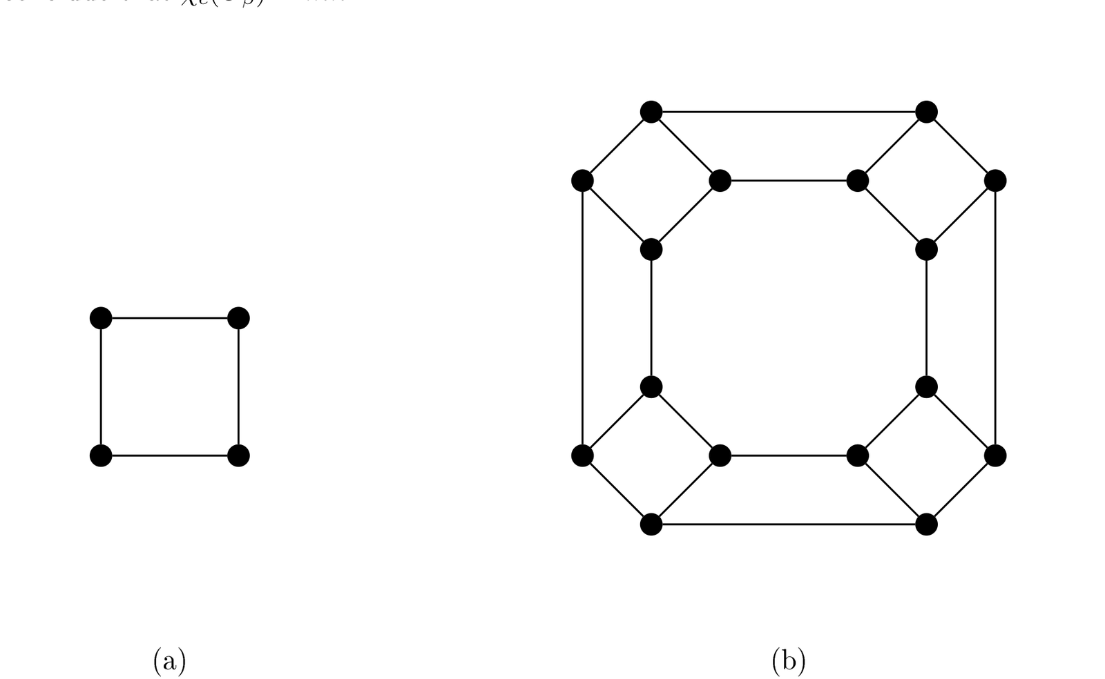
5. Cubic Inflation
For the notation for cubic inflation, we follow [2]. Let \(G\) be a graph without vertices of degree one. First, we replace each vertex \(v\in V(G)\) by a cycle \(C_v\) of length \(2deg(v)\), and then replace every edge \(uv\) of \(G\) by two edges joining \(C_u\) and \(C_v\). The resulting graph is called the cubic inflation of G. Order of \(CI(G)\) is \(\sum\limits_{v \in V(G)} 2{\deg(v)}\). Figure 5 illustrates cycle of order \(4\) and cubic inflation of cycle.
Theorem 5.1. Let \(G=C_n\) be a cycle graph on \(n\) vertices. Then
Proof. Let \(G = C_n\) be a cycle graph on \(n\) vertices where \(V(G)=\{v_1,v_2, \cdots,v_n\}\). After applying cubic inflation, each vertex \(v_i\) is replaced by the cycle \(C_4\) where the vertices are labeled as \(v_i^1,v_i^2,v_i^3,v_i^4\). Also the edges are defined as follows: for each \(1 \leq i \leq n-1\), the vertex \(v_i^1\) is adjacent to \(v_{i+1}^4\), and \(v_i^2\) is adjacent to \(v_{i+1}^3\). In addition, \(v_n^1\) is adjacent to \(v_1^4\), and \(v_n^2\) is adjacent to \(v_1^3\). We know that \(\chi_c(CI(G)) \leq 3\).
Case 1. \(n \equiv 0\pmod{3}\). Let \(c:V(CI(G)) \rightarrow [3]\) be a coloring defined as follows.
This coloring ensures that all three colors appear in the neighborhood of each vertex, thereby satisfying the coupon coloring condition.
Case 2. \(n \not \equiv 0\pmod{3}\). Suppose that a \(3\)-coupon coloring \(c : V(CI(G)) \to [3]\) exists. Consider the vertex \(v_1^4\), whose neighbors are \(v_1^3\), \(v_1^1\), and \(v_n^1\). Since \(c\) is a \(3\)-coupon coloring, \(c(v_1^3) \in \{1,2,3\}\). Without loss of generality, assume that \(c(v_1^1)=1\) and \(c(v_1^3)=2\). Then it follows that \(c(v_n^1)=3\), which in turn implies that \(c(v_n^3)=1\). Continuing like this we have \(2\) cases.
Case 2.1. \(n \equiv 1\pmod{3}\).
The vertex \(v_2^4\) becomes a bad vertex because its neighborhood does not contain all three colors.
Case 2.2. \(n \equiv 2\pmod{3}\).
The vertex \(v_1^2\) becomes a bad vertex because its neighborhood does not contain all three colors. Thus when \(n \not \equiv 0\pmod{3}\), \(\chi_c(CI(G)) \leq 2\). Define a coloring \(c: V(CI(G)) \rightarrow [2]\) as follows
Clearly, \(c\) is a coupon coloring. \(\square\)
Theorem 5.2. Let \(G=W_n\) be a wheel graph on \(n\) vertices. Then \(\chi_{c}(CI(G))=2\).
Proof. Let \(G=W_n\) be a wheel graph on \(n\) vertices with vertex set \(\{v_1, v_2, \ldots, v_n\}\), where \(v_1\) serves as the universal vertex. After applying cubic inflation, each vertex \(v_i, i=2,3,\cdots ,n\) is replaced by the cycle \(C_6\) with vertices labeled as \(v_i^1,v_i^2, \cdots, v_i^6\) and the vertex \(v_1\) is replaced by cycle \(C_{2(n-1)}\) with vertices labeled as \(v_1^1,v_1^2, \cdots ,v_1^{2(n-1)}\). In \(CI(G)\) the vertices \(v_1^{2i-1}\) is adjacent to \(v_{i+1}^1\) and \(v_1^{2i}\) is adjacent to \(v_{i+1}^2\) where \(i=1,2,\cdots,n-1\). Also, for every \(i = 2,3,\ldots,n-1\), the vertex \(v_i^{3}\) is adjacent to \(v_{i+1}^{6}\), while \(v_i^{4}\) is adjacent to \(v_{i+1}^{5}\). Also the vertices \(v_n^3\) and \(v_n^4\) are adjacent to \(v_2^6\) and \(v_2^5\) respectively. Since \(\delta(CI(G))=3\) we have \(\chi_c(CI(G))\leq 3\). Assume there exists a \(3-\)coupon coloring \(c:V(CI(G))\rightarrow [3]\). Consider the vertex \(v_2^5\) which is adjacent to \(v_2^4\), \(v_2^6\) and \(v_n^4\). Suppose \(c(v_2^4)=a\), \(a \in \{1,2,3\}\). Without loss of generality, assume that \(c(v_2^4)=1\), \(c(v_2^6)=2\) and \(c(v_n^4)=3\). Now consider the vertex \(v_n^3\), we get \(c(v_n^2)=1\). The neighboring vertices of the vertex \(v_1^{2n-2}\) are \(v_n^2\), \(v_1^1\) and \(v_1^{2n-1}\). The vertex \(v_1^1\) will receive either color \(2\) or \(3\). If \(v_1^1\) is assigned the color \(2\), then \(v_2^1\) becomes bad vertex since it will have two neighbors with the same color \(2\) and this will result in lack of three required colors in the neighborhood of \(v_2^1\). Hence, we must have \(c(v_1^1)=3\) and \(c(v_1^{2n-1})=2\). Finally considering the vertex \(v_n^1\), we obtain \(c(v_n^6)=3\) which causes \(v_n^5\) to become a bad vertex. Thus, \(\chi_c(CI(G)) \leq 2\). It now suffices to show that \(\chi_c(CI(G)) \geq 2\) by defining a \(2\)-coupon coloring of the graph \(CI(G)\). We define \(c:V(CI(G)) \rightarrow [2]\) as follows. Set \(c(v_1^i)=2\) for all \(i\) and for each \(j=2,3, \cdots, n\) \(c(v_j^1)=c(v_j^2)=1\), \(c(v_j^3)=c(v_j^6)=2\) and \(c(v_j^5)=c(v_j^4)=1\). Consider the vertices on larger cycle replacing the universal vertex that is \(v_1^i\), \(1 \le i \le 2(n-1)\), these vertices has the color \(2\) among themselves. So each vertex will have color \(2\) in its neighborhood. Also \(v_1^{2i-1}\) is adjacent to \(v_{i+1}^1\) and \(v_1^{2i}\) is adjacent to \(v_{i+1}^2\) and by the coloring pattern \(c(v_j^1)=c(v_j^2)=1\) for any \(j\) and hence any arbitrary \(v_1^i, 1 \le i \le 2(n-1)\) is adjacent to vertices which has color \(1\). Now for \(2 \le l \le 5\), consider the vertices \(v_j^l, 2 \le j \le n\) and these vertices will receive the required two colors from their adjacent vertices in the same cycle. For \(v_j^1\) and \(v_j^6\) these vertices are connected to vertices having color \(2\) and they receive the color \(1\) from the adjacent vertices in the same cycle. It can be easily seen that \(c\) is a coupon coloring. Thus \(\chi_c(CI(G))=2\). \(\square\)
6. Conclusion and future work
In this paper, we explored coupon coloring of inflated graphs and introduced new graph operations derived from inflation and analyzed their impact on coupon coloring. This can also be extended to other classes of graphs to study how these operations behave under varying structural properties.
Acknowledgment
The first author expresses her gratitude to Vellore Institute of Technology for providing financial support that enabled her to perform the research work.