
Throughout this paper, all graphs are finite, undirected, simple, and connected. For a graph \(G=(V(G),E(G))\) with \(V(G)=\{v_1,\dots,v_n\}\), we write \(n=|V(G)|\) for its order and \(d_G(v)\) (or simply \(d(v)\)) for the degree of a vertex \(v\in V(G)\). Let \(\delta(G)=\min\{d(v):v\in V(G)\}\) denote the minimum degree of \(G\). A vertex \(v\in V(G)\) is called a pendant vertex if \(d(v)=1\). Let \(N(u)\) denote the set of neighbours of \(u\). The adjacency matrix of \(G\) is denoted by \(A(G)=[a_{ij}]\) where \(a_{ij}=1\) if \(v_i\) is adjacent to \(v_j\), and \(a_{ij}=0\) otherwise. And let \(D(G)=\mathrm{diag}(d(v_1),\dots,d(v_n))\) be the diagonal degree matrix. The normalized Laplacian of \(G\) is defined by \[\mathcal{L}(G)=I_n-D(G)^{-1/2}A(G)D(G)^{-1/2},\] where \(I_n\) is the identity matrix of order \(n\). Since \(\mathcal{L}(G)\) is real symmetric, all its eigenvalues are real; we denote the largest eigenvalue by \(\rho(\mathcal{L}(G))\) and refer to it as the spectral radius of \(G\).
For \(n\ge 5\), let \(\mathcal{F}_n\) denote the family of connected simple graphs \(G\) of order \(n\) such that exactly one vertex of \(G\) has degree greater than two. For \(n\ge 6\), let \(\mathcal{G}_n\) denote the family of connected simple graphs \(G\) of order \(n\) such that exactly two vertices of \(G\) have degree greater than two.
The normalized Laplacian, introduced by Chung [3], plays an important role in spectral graph theory. In recent years, considerable attention has been paid to its spectral properties. Bounds for normalized Laplacian eigenvalues were obtained in [11]. The normalized Laplacian spectrum of complete multipartite graphs and the multiplicities of normalized Laplacian eigenvalues were studied in [16, 17], respectively. Other related topics include the spectral gap of the largest normalized Laplacian eigenvalue [10], the second largest normalized Laplacian eigenvalue [24], graphs with limited normalized algebraic connectivity [18], isospectral graphs [6], and spectral characterization with respect to the normalized Laplacian [19].
Extremal problems for normalized Laplacian eigenvalues form an active topic in this area. Das and Sun [5] investigated extremal graphs for the normalized Laplacian spectral radius and energy. For non-bipartite graphs, Guo, Li and Shiu characterized the graphs with largest normalized Laplacian spectral radius [9] and studied perturbation effects on this parameter in [8]. Further extremal results for normalized Laplacian spectral radii were obtained by Sun and Chen [15]. These results reveal that extremal normalized Laplacian spectral radii are strongly influenced by the structural constraints imposed on graphs.
The closest previous extremal results on normalized Laplacian spectral radii are those in [5, 8, 9, 15]. These papers deal with general graph classes, non-bipartite graphs, or perturbations and graph transformations under different structural assumptions. The problem studied here is of a different nature: the admissible graphs are prescribed by the exact number of vertices whose degrees are greater than two. This additional restriction changes the possible extremal structures and leads to minimizers which do not follow directly from the previously known extremal families.
Besides the general extremal theory for normalized Laplacian eigenvalues, there is also a substantial spectral literature on graphs and trees with very few branching vertices. In the Laplacian setting, starlike trees, namely trees with exactly one vertex of degree greater than two, were shown to be determined by their Laplacian spectrum [13], while double starlike trees and related families were studied from the same viewpoint in subsequent works [12, 14]. On the normalized Laplacian side, characteristic polynomials and explicit formulas were derived for trees, including starlike trees and certain double-starlike families [1]. From the viewpoint of the Laplacian spectral radius, trees with prescribed diameter, degree sequence, and maximum degree have also been extensively investigated [7, 21, 22, 23]. These results indicate that the number and arrangement of branching vertices strongly affect the extremal behavior of Laplacian-type spectral radii. Therefore, it is natural to study the normalized Laplacian spectral radius under restrictions on the number of vertices of degree greater than two.
The present problem is also distinct from the spectral results on starlike and double-starlike trees. Those works mainly concern spectral determination, characteristic polynomials, or the ordinary Laplacian spectral radius of trees. In this paper the matrix is the normalized Laplacian, and the graphs under consideration are connected simple graphs which may contain cycles. The restriction on the number of branching vertices therefore leads to different minimizers. For one branching vertex, the extremal graphs are formed by triangles sharing a common vertex, with an additional pendant vertex in the even-order case. For two branching vertices, the relation between the two branching vertices, their common neighbors, and the degree-two vertices produces different extremal families in odd and even orders. These features require structural reductions excluding long induced paths and pendant configurations, together with Rayleigh–Ritz estimates, interlacing, and equitable partitions.
In this paper, we determine the minimum of \(\rho(\mathcal{L}(G))\) over \(\mathcal{F}_n\) for all \(n\ge5\), over \(\mathcal{G}_n\) for odd \(n\ge7\), and over \(\mathcal{G}_n\) for even \(n\ge6\). For \(\mathcal{F}_n\), we determine the unique graph with minimum normalized Laplacian spectral radius and the corresponding exact minimum value. For \(\mathcal{G}_n\), we determine all extremal graphs when \(n\) is odd, and the unique extremal graph up to isomorphism when \(n\) is even, together with the exact minimum value.
Let \(G\) be a simple connected graph with adjacency matrix \(A\) and degree matrix \(D\). Define \[S=D^{-1/2}AD^{-1/2}, \qquad \mathcal{L}=I-S,\] where \(S\) is the normalized adjacency matrix of \(G\) and \(\mathcal{L}\) is the normalized Laplacian matrix of \(G\). Throughout this paper, \(\lambda\) and \(\mu\) denote eigenvalues of \(\mathcal{L}\) and \(S\), respectively. Since \(\mathcal{L}=I-S\), the spectra of \(S\) and \(\mathcal{L}\) satisfy \[\mathrm{Spec}(\mathcal{L})=\{\,1-\mu:\mu\in\mathrm{Spec}(S)\,\}.\]
In particular, \[\rho(\mathcal{L}(G))=\lambda_{\max}(\mathcal{L})=1-\mu_{\min}(S).\tag{1}\]
By the Rayleigh–Ritz principle, \[\mu_{\min}(S)=\min_{\mathbf{x}\neq \mathbf{0}}\frac{\mathbf{x}^{T}S\mathbf{x}}{\mathbf{x}^{T}\mathbf{x}}, \qquad \rho(\mathcal{L})=\lambda_{\max}(\mathcal{L}) =\max_{\mathbf{f}\neq \mathbf{0}}\frac{\mathbf{f}^{T}\mathcal{L}\mathbf{f}}{\mathbf{f}^{T}\mathbf{f}}.\tag{2}\]
Moreover, by setting \(\mathbf{g}=D^{-1/2}\mathbf{f}\), we obtain \[\rho(\mathcal{L}) =\max_{\mathbf{g}\neq \mathbf{0}} \frac{\sum_{ij\in E(G)}(g_i-g_j)^2} {\sum_{i\in V(G)} d(i) g_i^2}.\tag{3}\]
Let \(P_r\) denote the path graph on \(r\) vertices. A simple path of length \(r-1\) in \(G\) is a sequence of distinct vertices \(u_1u_2\cdots u_r\) such that \(u_i u_{i+1}\in E(G)\) for \(i=1,2,\dots,r-1\).
For a finite set \(X\), let \(\mathbb R^X\) denote the real vector space of all real-valued functions on \(X\). In particular, \(\mathbb R^{V(G)}\) is the vector space of real-valued functions on the vertex set of \(G\).
For a vertex subset \(T \subseteq V(G)\), let \(\mathbf{1}_T \in \mathbb{R}^{V(G)}\) denote vector \[(\mathbf{1}_T)_u= \begin{cases} 1, & u\in T,\\ 0, & u\notin T. \end{cases}\]
For a vertex \(v \in V(G)\), let \(e_v \in \mathbb{R}^{V(G)}\) denote the vector \(\mathbf{1}_{\{v\}}\).
Lemma 2.1. [2] Let \(A\) be a real symmetric matrix of order \(n\), and let \(B\) be a principal submatrix of \(A\) of order \(m\) (\(m < n\)). Then the eigenvalues of \(B\) interlace with the eigenvalues of \(A\). In particular, the minimum eigenvalue of \(A\) is bounded above by the minimum eigenvalue of \(B\), that is, \[\lambda_{\min}(A) \le \lambda_{\min}(B).\]
Lemma 2.2. [4] Let \(M\) be a block matrix given by \(M = \begin{pmatrix} A & B \\ C & D \end{pmatrix}\), where \(A, B, C, D\) are the \(p \times p, p \times q, q \times p, q \times q\) matrices, with \(A\) and \(D\) being invertible. Then \[\det(M) = \det(A) \det(D – C A^{-1} B) = \det(D) \det(A – B D^{-1} C).\]
Lemma 2.3. [3] Let \(G\) be a connected bipartite graph, and let \(\mathcal{L}(G)\) be the normalized Laplacian matrix of \(G\). Then \[\rho(\mathcal{L}(G))=\lambda_{\max}(\mathcal{L}(G))=2.\]
Let \(M=(m_{uv})\) be a real symmetric matrix, and let \(\Pi=\{C_1,\dots,C_k\}\) be a partition of its index set. If for any \(i,j\in\{1,\dots,k\}\) and any \(u,v\in C_i\), \[\sum_{w\in C_j} m_{uw}=\sum_{w\in C_j} m_{vw},\] then \(\Pi\) is called an equitable partition of \(M\). In this case, the matrix \(Q=(q_{ij})\) defined by \[q_{ij}=\sum_{w\in C_j} m_{uw},\qquad u\in C_i,\] is well defined, and is called the quotient matrix of \(M\) with respect to \(\Pi\).
Lemma 2.4. [20] Let \(\Pi\) be an equitable partition of a real symmetric matrix \(M\), and let \(Q\) be the corresponding quotient matrix. Then \[\mathrm{Spec}(Q)\subseteq \mathrm{Spec}(M).\]
In this section, we determine the graph with minimum normalized Laplacian spectral radius in \(\mathcal{F}_n(n\geq5)\). We first present a candidate extremal graph, and then derive several structural properties that any extremal graph in \(\mathcal{F}_n\) must satisfy. These results lead to a complete characterization of the extremal graph in \(\mathcal{F}_n\).
Before presenting our first result, we recall the definition of the join of two graphs. Let \(G\) and \(H\) be two vertex-disjoint graphs, the join of \(G\) and \(H\), denoted by \(G \vee H\), is the graph obtained from the disjoint union \(G \cup H\) by adding all edges between \(V(G)\) and \(V(H)\).
For \(n\ge 5\), define the graph \(H_n\) as follows.
(i) If \(n=2m+1\) for some integer \(m\ge 2\), let \(H_n=H_{2m+1}:=mK_2\vee K_1,\) where \(V(K_1)=\{v_0\}\); see the left graph in Figure 1.
(ii) If \(n=2m+2\) for some integer \(m\ge 2\), let \(H_n=H_{2m+2}\), be the graph obtained from \(H_{2m+1}\) by attaching a new pendant vertex \(\ell\) to the central vertex \(v_0\); see the right graph in Figure 1.
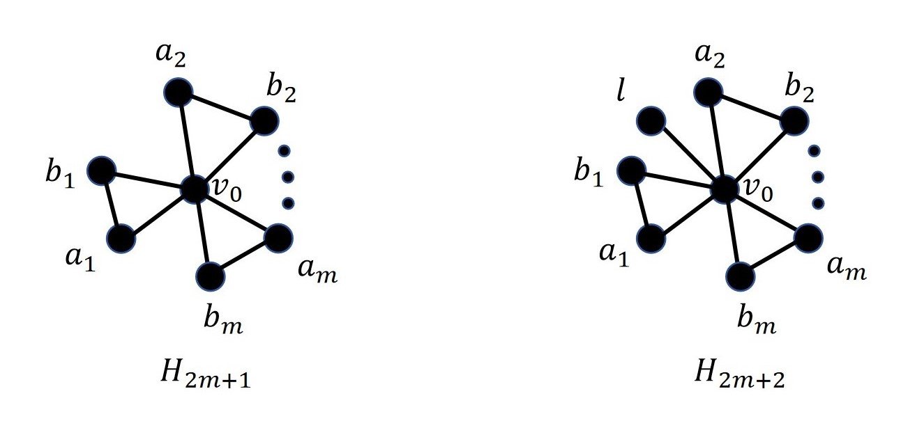
Proposition 3.1. For \(m \geq 2\), let \(H_{2m+1}\) and \(H_{2m+2}\) be the graphs defined above. The normalized Laplacian spectrum of \(H_n\) is given by:
(i) If \(n = 2m+1\), then \[\operatorname{Spec}(\mathcal{L}(H_{2m+1})) = \left\{ 0^{(1)}, \left(\frac{1}{2}\right)^{(m-1)}, \left(\frac{3}{2}\right)^{(m+1)} \right\}.\]
(ii) If \(n=2m+2\), and \(d=d(v_0)=2m+1=n-1\). Then \[\operatorname{Spec}(\mathcal{L}(H_{2m+2})) = \left\{ 0^{(1)}, \left(\frac{1}{2}\right)^{(m-1)}, \left(\frac{3}{2}\right)^{(m)}, \lambda_{+}^{(1)}, \lambda_{-}^{(1)} \right\},\] where \(\lambda_{\pm} = \frac{5}{4} \mp \frac{1}{4} \sqrt{1 + \frac{8}{n-1}}.\)
Proof. We determine the spectrum of the normalized adjacency matrix \(S\).
For each \(i\in\{1,\dots,m\}\), let \(a_i\) and \(b_i\) be the two non-central vertices of the \(i\)-th triangle. Then \[d(a_i)=d(b_i)=2.\]
Moreover, \[d(v_0)=2m \quad \text{in } H_{2m+1}, \qquad d(v_0)=2m+1=n-1=:d \quad \text{in } H_{2m+2},\] and in the even case \[d(\ell)=1.\]
For each \(i\in\{1,\dots,m\}\), define \[\mathbf{u}_i=\mathbf{e}_{a_i}-\mathbf{e}_{b_i}.\]
Since \[S\mathbf{e}_{a_i}=\frac12\mathbf{e}_{b_i} +\frac{1}{\sqrt{2d(v_0)}}\mathbf{e}_{v_0}, \qquad S\mathbf{e}_{b_i}=\frac12\mathbf{e}_{a_i} +\frac{1}{\sqrt{2d(v_0)}}\mathbf{e}_{v_0},\] we have \[S\mathbf{u}_i=-\frac12 \mathbf{u}_i .\]
Thus the subspace \[W_-=\operatorname{span}\{\mathbf{u}_1,\ldots,\mathbf{u}_m\},\] is \(S\)-invariant, \(S|_{W_-}=-\frac12 I\), and \(\dim W_-=m\). Hence \(-\frac12\) is an eigenvalue of \(S\) with multiplicity at least \(m\).
Next, let \[\mathbf{s}_i=\mathbf{e}_{a_i}+\mathbf{e}_{b_i}, \qquad W_T=\left\{\sum_{i=1}^m c_i \mathbf{s}_i:\sum_{i=1}^m c_i=0\right\}.\]
For each \(i\), \[S\mathbf{s}_i =\frac12\mathbf{s}_i+\frac{2}{\sqrt{2d(v_0)}}\mathbf{e}_{v_0}.\]
Therefore, if \(\mathbf{x}=\sum_{i=1}^m c_i\mathbf{s}_i\in W_T\), then \[S\mathbf{x} =\frac12\sum_{i=1}^m c_i\mathbf{s}_i +\frac{2}{\sqrt{2d(v_0)}}\left(\sum_{i=1}^m c_i\right)\mathbf{e}_{v_0} =\frac12\mathbf{x}.\]
Thus \(W_T\) is \(S\)-invariant, \(S|_{W_T}=\frac12 I\), and \(\dim W_T=m-1\). Hence \(\frac12\) is an eigenvalue of \(S\) with multiplicity at least \(m-1\).
It remains to determine the remaining eigenvalues.
Case 1. \(n=2m+1\).
Let \[T=\{a_i,b_i:1\le i\le m\}, \qquad \mathbf{x}_0=\mathbf{e}_{v_0}, \qquad \mathbf{x}_1=\frac{1}{\sqrt{2m}}\mathbf{1}_T.\]
Then the subspace \[U=\mathrm{Span}\{\mathbf{x}_0,\mathbf{x}_1\},\] is invariant under \(S\). Moreover, \[\mathbb R^{V(H_{2m+1})}=W_-\oplus W_T\oplus U,\] is an orthogonal direct sum. Indeed, for all \(i,j\), \[\langle \mathbf{u}_i,\mathbf{s}_j\rangle=0,\qquad \langle \mathbf{u}_i,\mathbf{e}_{v_0}\rangle=0,\qquad \langle \mathbf{u}_i,\mathbf{1}_T\rangle=0.\]
Moreover, if \(\mathbf{x}=\sum_{i=1}^m c_i\mathbf{s}_i\in W_T\), then \[\langle \mathbf{x},\mathbf{e}_{v_0}\rangle=0,\qquad \langle \mathbf{x},\mathbf{1}_T\rangle=2\sum_{i=1}^m c_i=0.\]
Thus \(W_-\), \(W_T\), and \(U\) are mutually orthogonal. Since \[\dim W_-+\dim W_T+\dim U=m+(m-1)+2=2m+1=|V(H_{2m+1})|,\] their orthogonal sum is the whole space \(\mathbb R^{V(H_{2m+1})}\).
With respect to the orthonormal basis \(\{\mathbf{x}_0,\mathbf{x}_1\}\), the matrix of \(S|_U\) is \[B= \begin{pmatrix} 0 & \frac{1}{\sqrt{2}}\\[2mm] \frac{1}{\sqrt{2}} & \frac12 \end{pmatrix}.\]
Hence \[\det(\mu I-B) = \begin{vmatrix} \mu & -\frac1{\sqrt2}\\[1mm] -\frac1{\sqrt2} & \mu-\frac12 \end{vmatrix} =\mu\left(\mu-\frac12\right)-\frac12 =(\mu-1)\left(\mu+\frac12\right).\]
Therefore the eigenvalues of \(B\) are \[1,\,-\frac12.\]
Since \[m+(m-1)+2=2m+1=|V(H_{2m+1})|,\] we have obtained the whole spectrum of \(S\). Thus \[\mathrm{Spec}(S(H_{2m+1}))= \left\{ 1^{(1)}, \left(\frac12\right)^{(m-1)}, \left(-\frac12\right)^{(m+1)} \right\}.\]
Therefore, \[\mathrm{Spec}(\mathcal{L}(H_{2m+1}))= \left\{ 0^{(1)}, \left(\frac12\right)^{(m-1)}, \left(\frac32\right)^{(m+1)} \right\}.\]
Case 2. \(n=2m+2\).
Let \[P=\{\ell\}, \qquad T=\{a_i,b_i:1\le i\le m\}, \qquad \mathbf{x}_0=\mathbf{e}_{v_0}, \qquad \mathbf{x}_1=\mathbf{e}_{\ell}, \qquad \mathbf{x}_2=\frac{1}{\sqrt{2m}}\mathbf{1}_T.\]
Then the subspace \[U=\mathrm{Span}\{\mathbf{x}_0,\mathbf{x}_1,\mathbf{x}_2\},\] is invariant under \(S\). Moreover, \[\mathbb R^{V(H_{2m+2})}=W_-\oplus W_T\oplus U,\] is an orthogonal direct sum. The orthogonality between \(W_-\) and \(W_T\) is the same as in the odd case. Also \(W_-\) is orthogonal to \(\mathbf{e}_{v_0}\), \(\mathbf{e}_{\ell}\), and \(\mathbf{1}_T\). If \(\mathbf{x}=\sum_{i=1}^m c_i\mathbf{s}_i\in W_T\), then \[\langle \mathbf{x},\mathbf{e}_{v_0}\rangle= \langle \mathbf{x},\mathbf{e}_{\ell}\rangle=0,\qquad \langle \mathbf{x},\mathbf{1}_T\rangle=2\sum_{i=1}^m c_i=0.\]
Thus \(W_-\), \(W_T\), and \(U\) are mutually orthogonal. Since \[\dim W_-+\dim W_T+\dim U=m+(m-1)+3=2m+2=|V(H_{2m+2})|,\] their orthogonal sum is the whole space \(\mathbb R^{V(H_{2m+2})}\).
With respect to the orthonormal basis \(\{\mathbf{x}_0,\mathbf{x}_1,\mathbf{x}_2\}\), the matrix of \(S|_U\) is \[B= \begin{pmatrix} 0 & \frac{1}{\sqrt d} & \sqrt{\frac{m}{d}}\\[2mm] \frac{1}{\sqrt d} & 0 & 0\\[2mm] \sqrt{\frac{m}{d}} & 0 & \frac12 \end{pmatrix}.\]
Thus \[\begin{aligned} \det(\mu I-B) &= \begin{vmatrix} \mu & -\frac1{\sqrt d} & -\sqrt{\frac md}\\[1mm] -\frac1{\sqrt d} & \mu & 0\\[1mm] -\sqrt{\frac md} & 0 & \mu-\frac12 \end{vmatrix} \\ &=\mu^2\left(\mu-\frac12\right) -\frac{1}{d}\left(\mu-\frac12\right) -\frac{m}{d}\mu \\ &=(\mu-1)\left(\mu^2+\frac12\mu-\frac{1}{2d}\right), \end{aligned}\] where in the last equality we use \(d=2m+1\). Therefore the eigenvalues of \(B\) are \[1,\qquad \mu_{\pm}=\frac{-1\pm\sqrt{1+\frac{8}{d}}}{4} =\frac{-1\pm\sqrt{1+\frac{8}{n-1}}}{4}.\]
Since \[m+(m-1)+3=2m+2=|V(H_{2m+2})|,\] we have obtained the whole spectrum of \(S\). Hence \[\mathrm{Spec}(S(H_{2m+2}))= \left\{ 1^{(1)}, \left(\frac12\right)^{(m-1)}, \left(-\frac12\right)^{(m)}, \mu_+^{(1)}, \mu_-^{(1)} \right\}.\]
Therefore, \[\mathrm{Spec}(\mathcal{L}(H_{2m+2}))= \left\{ 0^{(1)}, \left(\frac12\right)^{(m-1)}, \left(\frac32\right)^{(m)}, \lambda_+^{(1)}, \lambda_-^{(1)} \right\},\] where \[\lambda_{\pm}=1-\mu_{\pm} =\frac54\mp\frac14\sqrt{1+\frac{8}{n-1}}.\]
This completes the proof. \(\square\)
Corollary 3.2. Let \(n\ge 5\), and let \(H_n\) be the graph defined above. Then the spectral radius of the normalized Laplacian matrix of \(H_n\) satisfies \(\rho(\mathcal{L}(H_n))<1+\frac{\sqrt2}{2}.\)
Proof. First assume that \(n=2m+1\) is odd. By Proposition 3.1(i), \[\rho(\mathcal{L}(H_n))=\frac32.\]
Since \(\frac32<1+\frac{\sqrt2}{2},\) the desired inequality follows.
Now assume that \(n=2m+2\) is even, and set \(d=n-1.\) Then \(d\ge 5\). By Proposition 3.1(ii), \[\rho(\mathcal{L}(H_n))=\frac54+\frac14\sqrt{1+\frac8d}.\]
Consider the function \[f(x)=\frac54+\frac14\sqrt{1+\frac8x}, \qquad x>0.\]
The function \(\sqrt{1+\frac{8}{x}}\) is strictly decreasing on \((0,\infty)\). Therefore, \(f\) is also strictly decreasing on \((0,\infty)\). Hence, by \(d\ge 5\), we obtain \[\rho(\mathcal{L}(H_n))=f(d)\le f(5)=\frac54+\frac14\sqrt{\frac{13}{5}}.\] it is easy to see that \(\frac54+\frac14\sqrt{\frac{13}{5}}<1+\frac{\sqrt2}{2}.\) Therefore \[\rho(\mathcal{L}(H_n)) \le \frac54+\frac14\sqrt{\frac{13}{5}} <1+\frac{\sqrt2}{2}.\] \(\square\)
Lemma 3.3. Let \(G\in\mathcal{F}_n\) be a non-bipartite graph, then the spectral radius of its normalized Laplacian matrix satisfies \(\rho(\mathcal{L}(G)) \geq \frac{3}{2}.\)
Proof. By Eq. (1), we have \(\rho(\mathcal{L}(G))=\lambda_{\max}(\mathcal{L})=1-\mu_{\min}(S).\) Therefore, it suffices to show that \[\mu_{\min}(S)\le -\frac12.\]
Since \(G\) is non-bipartite, it contains an odd cycle. Let \(v_0\) denote the unique vertex of \(G\) with degree greater than \(2\). We first show that every odd cycle of \(G\) contains \(v_0\). Suppose that there exists an odd cycle \(C\) with \(v_0\notin V(C)\). Then every vertex of \(C\) has degree at most \(2\), because every vertex other than \(v_0\) has degree at most \(2\) in \(\mathcal{F}_n\). On the other hand, each vertex of \(C\) already has two neighbors on the cycle, and hence every vertex of \(C\) has degree exactly \(2\). It follows that no vertex of \(C\) is adjacent to a vertex outside \(C\), so \(C\) is a connected component of \(G\), contradicting the connectedness of \(G\). Thus every odd cycle of \(G\) contains \(v_0\).
Let \(C\) be an odd cycle of \(G\). Since \(|V(C)|\ge 3\), \(C\) contains an edge \(xy\) not incident with \(v_0\). Hence \(x,y\ne v_0\), so \(d(x),d(y)\le 2\). On the other hand, both \(x\) and \(y\) already have two neighbors on \(C\). Therefore, \(d(x)=d(y)=2.\)
Define \(\mathbf{f}\in \mathbb{R}^{V(G)}\) by \[f(v)= \begin{cases} \sqrt{d(x)}, & v=x,\\ -\sqrt{d(y)}, & v=y,\\ 0, & \text{otherwise}. \end{cases}\]
Then \(\mathbf{f}\neq 0\), and since \(d(x)=d(y)=2\) and \(xy\in E(G)\), \[\mathbf{f}^{T}\mathbf{f}=d(x)+d(y)=4,\qquad \mathbf{f}^{T}S\mathbf{f}=2S_{xy}f(x)f(y) =2\cdot \frac{1}{\sqrt{d(x)d(y)}}\cdot \sqrt{d(x)}\,(-\sqrt{d(y)})=-2.\]
Hence, by Eq. (2), \[\mu_{\min}(S)\le \frac{\mathbf{f}^{T}S\mathbf{f}}{\mathbf{f}^{T}\mathbf{f}}=-\frac12.\] Therefore, \(\rho(\mathcal{L}(G))=1-\mu_{\min}(S)\ge \frac32.\) \(\square\)
For a graph \(G\) and \(U\subseteq V(G)\), let \(G[U]\) denote the subgraph induced by \(U\), that is, the graph with vertex set \(U\) and edge set \(E(G[U])=\{uv\in E(G):u,v\in U\}.\) A graph \(H\) is an induced subgraph of \(G\) if \(H=G[U]\) for some \(U\subseteq V(G)\). An induced path in \(G\) is a path \(u_1u_2\cdots u_r\) such that \(G[\{u_1,u_2,\ldots,u_r\}] \cong P_r.\)
Lemma 3.4. Let \(G\) be a graph containing an induced path \(u_1u_2\cdots u_r, r\ge 3,\) such that \(d(u_k)=2, k=1,\ldots,r.\) Then \(\mu_{\min}(S)\le -\cos\frac{\pi}{r+1}.\) Consequently, \(\rho(\mathcal{L}(G))\ge 1+\cos\frac{\pi}{r+1}.\) In particular, when \(r=3\), \(\rho(\mathcal{L}(G))\ge 1+\frac{\sqrt2}{2}.\)
Proof. Let \(\alpha=\dfrac{\pi}{r+1}\), and define \(\mathbf{x}\in \mathbb{R}^{V(G)}\) by \[x(v)= \begin{cases} (-1)^k\sin(k\alpha), & v=u_k,\ k=1,\dots,r,\\ 0, & \text{otherwise}. \end{cases}\]
Then \(\mathbf{x}\neq 0\). By Eq. (2), \(\mu_{\min}(S)\le \frac{\mathbf{x}^{T}S\mathbf{x}}{\mathbf{x}^{T}\mathbf{x}}.\)
Since \(u_1u_2\cdots u_r\) is an induced path and \(d(u_k)=2\) for all \(k\), the only nonzero off-diagonal entries of \(S\) on \(\{u_1,\dots,u_r\}\) are \[S_{u_ku_{k+1}}=\frac{1}{\sqrt{d(u_k)d(u_{k+1})}}=\frac12, \qquad k=1,\dots,r-1.\]
Hence \[\mathbf{x}^{T}\mathbf{x}=\sum_{k=1}^{r}\sin^{2}(k\alpha),\] and \[\mathbf{x}^{T}S\mathbf{x} =2\sum_{k=1}^{r-1}S_{u_ku_{k+1}}x(u_k)x(u_{k+1}) =-\sum_{k=1}^{r-1}\sin(k\alpha)\sin((k+1)\alpha).\]
Now let \[\mathbf{z}=(\sin\alpha,\sin(2\alpha),\dots,\sin(r\alpha))^{T}\in\mathbb{R}^{r}.\]
Since \(\mathbf{z}\) is an eigenvector of \(A(P_r)\) corresponding to the eigenvalue \(2\cos\alpha\). Therefore, \[2\sum_{k=1}^{r-1}\sin(k\alpha)\sin((k+1)\alpha) =\mathbf{z}^{T}A(P_r)\mathbf{z} =2\cos\alpha\, \mathbf{z}^{T}\mathbf{z} =2\cos\alpha\sum_{k=1}^{r}\sin^{2}(k\alpha).\]
Thus \[\mathbf{x}^{T}S\mathbf{x}=-\cos\alpha\, \mathbf{x}^{T}\mathbf{x},\] and so \[\mu_{\min}(S)\le \frac{\mathbf{x}^{T}S\mathbf{x}}{\mathbf{x}^{T}\mathbf{x}} =-\cos\alpha =-\cos\frac{\pi}{r+1}.\]
Consequently, \[\rho(\mathcal{L}(G))=1-\mu_{\min}(S)\ge 1+\cos\frac{\pi}{r+1}.\]
In particular, when \(r=3\), \(\rho(\mathcal{L}(G))\ge 1+\cos\frac{\pi}{4} =1+\frac{\sqrt2}{2}.\) \(\square\)
Corollary 3.5. Let \(G\in \mathcal{F}_n\) be an extremal graph. Then every cycle of \(G\) is a triangle. In particular, \(G\) contains no cycle of length at least \(4\).
Proof. Suppose, to the contrary, that \(G\) contains a cycle \(C\) of length \(\ell\ge 4\). Since \(G\in\mathcal F_n\), the unique vertex \(v_0\) of degree greater than \(2\) must lie on \(C\). Writing \(C=v_0u_1u_2\cdots u_{\ell-1}v_0,\) we see that \(u_1u_2\cdots u_{\ell-1}\) is an induced path on \(\ell-1\ge 3\) vertices. Moreover, for each \(i\), since \(u_i\ne v_0\), we have \(d(u_i)\le 2\), while \(u_i\) already has two neighbors on \(C\); hence \(d(u_i)=2\). By Lemma 3.4, \(\rho(\mathcal L(G))\ge 1+\cos\frac{\pi}{\ell}\ge 1+\cos\frac{\pi}{4} =1+\frac{\sqrt2}{2}.\) On the other hand, Corollary 3.2 yields a graph \(H_n\in\mathcal F_n\) such that \(\rho(\mathcal L(H_n))<1+\frac{\sqrt2}{2}.\) This contradicts the extremality of \(G\). Hence every cycle of \(G\) is a triangle. \(\square\)
Lemma 3.6. Let \(G\in \mathcal{F}_n\) be an extremal graph, and let \(v_0\) be the unique vertex of \(G\) with degree at least \(3\). If \(x\) is a pendant vertex of \(G\), then \(x\) is adjacent to \(v_0\).
Proof. Suppose, to the contrary, that \(x\) is a pendant vertex not adjacent to \(v_0\), and let \(u\) be the unique neighbor of \(x\). Then \(u\ne v_0\), so \(d(u)\le 2\). Since \(G\) is connected and \(x\) is pendant, \(u\) has a neighbor other than \(x\), and hence \(d(u)=2\).
Define \(\mathbf{f}\in \mathbb{R}^{V(G)}\) by \[f(v) = \begin{cases} 1, & \text{if } v = x, \\ -1, & \text{if } v = u, \\ 0, & \text{otherwise.} \end{cases}\]
Then \(\mathbf{f}\neq 0\), and since \(d(x)=1\), \(d(u)=2\), and \(xu\in E(G)\), \[\mu_{\min}(S)\le \frac{\mathbf{f}^{T}S\mathbf{f}}{\mathbf{f}^{T}\mathbf{f}} =\frac{2S_{xu}f(x)f(u)}{2} =-\frac{1}{\sqrt{d(x)d(u)}} =-\frac{\sqrt2}{2}.\]
Therefore, by Eq. (1), we have \(\rho(\mathcal{L}(G))=1-\mu_{\min}(S)\ge 1+\frac{\sqrt2}{2}.\) On the other hand, by Corollary 3.2, there exists \(H_n\in\mathcal{F}_n\) such that \(\rho(\mathcal{L}(H_n))<1+\frac{\sqrt2}{2}.\) This contradicts the extremality of \(G\). Hence \(x\) is adjacent to \(v_0\). \(\square\)
Lemma 3.7. Let \(G\in \mathcal{F}_n\) be an extremal graph. Then \(G\) has at most one pendant vertex.
Proof. By Corollary 3.2, there exists \(H_n\in\mathcal F_n\) such that \(\rho(\mathcal L(H_n))<2.\) Hence an extremal graph \(G\in\mathcal F_n\) is not bipartite, since every connected bipartite graph satisfies \(\rho(\mathcal L(G))=2\) by Lemma 2.3.
Let \(v_0\) be the unique vertex of \(G\) with degree greater than \(2\). By Corollary 3.5, every cycle of \(G\) is a triangle, and by Lemma 3.6, every pendant vertex is adjacent to \(v_0\). Therefore, \(G\) consists of \(m\ge 1\) triangles sharing the common vertex \(v_0\) and \(t\ge 0\) pendant vertices attached to \(v_0\). In particular, \(n=1+2m+t,\) and \(d(v_0)=2m+t=n-1=:d.\)
If \(t=0\), then \(G=H_{2m+1}\), and Proposition 3.1 gives \(\rho(\mathcal L(G))=\frac32.\) Thus it remains to consider the case \(t\ge 1\).
Now assume that \(t\ge 1\). Let \(P\) be the set of pendant vertices, and let \(T=\{a_i,b_i:1\le i\le m\}\) be the set of non-central vertices lying on the \(m\) triangles.
We determine the spectrum of the normalized adjacency matrix\(S\).
For the pendant part, define \[W_P=\left\{\mathbf{x}\in \mathbb{R}^{V(G)}: x(u)=0 \text{ for all } u\notin P,\ \sum_{u\in P}x(u)=0\right\}.\]
Then \(\dim W_P=t-1\). If \(\mathbf{x}\in W_P\), then for every pendant vertex \(p\in P\) we have \((S\mathbf{x})(p)=x(v_0)/\sqrt d=0\). At the central vertex, \[(S\mathbf{x})(v_0)=\frac1{\sqrt d}\sum_{p\in P}x(p)=0,\] and all remaining coordinates are zero because \(\mathbf{x}\) is supported on \(P\). Hence \[S\mathbf{x}=0 \qquad \text{for all } \mathbf{x}\in W_P.\]
Thus \(0\) is an eigenvalue of \(S\) with multiplicity at least \(t-1\).
For each \(i\in\{1,\dots,m\}\), let \[\mathbf{u}_i=\mathbf{e}_{a_i}-\mathbf{e}_{b_i}.\]
Then \[S\mathbf{u}_i=-\frac12 \mathbf{u}_i,\] and hence \(-\frac12\) is an eigenvalue of \(S\) with multiplicity at least \(m\).
Next, let \[\mathbf{s}_i=\mathbf{e}_{a_i}+\mathbf{e}_{b_i}, \qquad W_T=\left\{\sum_{i=1}^m c_i \mathbf{s}_i:\sum_{i=1}^m c_i=0\right\}.\]
Then \(\dim W_T=m-1\), and for every \(\mathbf{x}\in W_T\), \[S\mathbf{x}=\frac12 \mathbf{x}.\]
Hence \(\frac12\) is an eigenvalue of \(S\) with multiplicity at least \(m-1\).
It remains to determine the three remaining eigenvalues. Set \[\mathbf{x}_0=\mathbf{e}_{v_0}, \qquad \mathbf{x}_1=\frac{1}{\sqrt t}\mathbf 1_P, \qquad \mathbf{x}_2=\frac{1}{\sqrt{2m}}\mathbf 1_T.\]
Then the subspace \[U=\mathrm{Span}\{\mathbf{x}_0,\mathbf{x}_1,\mathbf{x}_2\},\] is invariant under \(S\). With respect to the orthonormal basis \(\{\mathbf{x}_0,\mathbf{x}_1,\mathbf{x}_2\}\), the matrix of \(S|_U\) is \[B= \begin{pmatrix} 0 & \sqrt{\dfrac td} & \sqrt{\dfrac md}\\[1mm] \sqrt{\dfrac td} & 0 & 0\\[1mm] \sqrt{\dfrac md} & 0 & \dfrac12 \end{pmatrix}.\]
We compute the characteristic polynomial explicitly: \[\begin{aligned} \det(\mu I-B) &= \begin{vmatrix} \mu & -\sqrt{\dfrac td} & -\sqrt{\dfrac md}\\[2mm] -\sqrt{\dfrac td} & \mu & 0\\[2mm] -\sqrt{\dfrac md} & 0 & \mu-\frac12 \end{vmatrix} \\ &=\mu^2\left(\mu-\frac12\right) -\frac{t}{d}\left(\mu-\frac12\right) -\frac{m}{d}\mu \\ &=\mu^3-\frac12\mu^2-\frac{m+t}{d}\mu+\frac{t}{2d}. \end{aligned}\]
Since \(d=2m+t\), this becomes \[\det(\mu I-B) =(\mu-1)\left(\mu^2+\frac12\mu-\frac{t}{2d}\right).\]
Therefore, the eigenvalues of \(B\) are \[1, \qquad \mu_\pm=\frac{-1\pm\sqrt{1+\frac{8t}{d}}}{4}.\]
Since \[(t-1)+m+(m-1)+3=2m+t+1=n,\] we have now obtained the whole spectrum of \(S\). In particular, \[\mu_{\min}(S)=\mu_-=\frac{-1-\sqrt{1+\frac{8t}{d}}}{4}.\]
By Eq. (1), \[\rho(\mathcal L(G)) =1-\mu_{\min}(S) =\frac54+\frac14\sqrt{1+\frac{8t}{d}}.\]
Since \(d=n-1\) is fixed, the right-hand side is strictly increasing in \(t\). On the other hand, the relation \[n=1+2m+t,\] implies that \(t\equiv n-1 \pmod 2\). Hence the smallest admissible value of \(t\) is \(0\) when \(n\) is odd, and \(1\) when \(n\) is even. Since \(G\) is extremal, \(t\) must be as small as possible. Therefore, \[t\le 1.\]
That is, \(G\) has at most one pendant vertex. \(\square\)
Theorem 3.8. Let \(n\ge 5\). Then the minimum normalized Laplacian spectral radius over \(\mathcal{F}_n\) is attained uniquely up to isomorphism, and is given as follows.
(i) If \(n=2m+1\), then \(\min_{G\in\mathcal{F}_n}\rho(\mathcal{L}(G))=\frac32,\) with equality if and only if \(G\cong H_{2m+1}.\)
(ii) If \(n=2m+2\), then \(\min_{G\in\mathcal{F}_n}\rho(\mathcal{L}(G)) = \frac54+\frac14\sqrt{1+\frac{8}{n-1}},\) with equality if and only if \(G\cong H_{2m+2}.\)
Proof. Let \(G\in\mathcal F_n\) be an extremal graph. By Corollary 3.2, there exists \(H_n\in\mathcal F_n\) such that \(\rho(\mathcal L(H_n))<1+\frac{\sqrt2}{2}.\) Since every connected bipartite graph satisfies \(\rho(\mathcal L(G))=2\) by Lemma 2.3, the graph \(G\) is not bipartite. And by Lemma 3.3, \(\rho(\mathcal{L}(G))\) satisfies \(\frac{3}{2}\leq \rho(\mathcal{L}(G))<1+\frac{\sqrt2}{2}.\)
Let \(v_0\) be the unique vertex of \(G\) with degree greater than \(2\). By Corollary 3.5, every cycle of \(G\) is a triangle; by Lemma 3.6, every pendant vertex of \(G\) is adjacent to \(v_0\); and by Lemma 3.7, \(G\) has at most one pendant vertex. It follows that \(G\) consists of \(m\) triangles sharing the common vertex \(v_0\), together with at most one pendant vertex attached to \(v_0\).
If \(n=2m+1\), then \(G\) has no pendant vertex, and hence \(G\cong H_{2m+1}.\) If \(n=2m+2\), then \(G\) has exactly one pendant vertex, and hence \(G\cong H_{2m+2}.\) Therefore, Proposition 3.1 yields \[\rho(\mathcal{L}(H_n))= \begin{cases} \dfrac32, & n=2m+1,\\[2mm] \dfrac54+\dfrac14\sqrt{1+\dfrac{8}{n-1}}, & n=2m+2. \end{cases}\] \(\square\)
In this section, we determine the graph with minimum normalized Laplacian spectral radius in \(\mathcal G_n\) \((n\ge 6)\). As in the previous section, we first introduce two special classes of graphs, see Figure 2. Recall that for two vertex-disjoint graphs \(G\) and \(H\), and vertices \(u\in V(G)\) and \(v\in V(H)\), \(G_{uv}H\) denotes the graph obtained from \(G\cup H\) by adding the edge \(uv\).
For \(n\ge 6\), define the graph \(G_n(a,b)\) as follows.
Let \(u\) and \(v\) be the central vertices of \(H_{2a+1}\) and \(H_{2b+1}\), respectively.
(i) If \(n=2m+2\) for some integer \(m\ge 2\), let \(a,b\ge 1\) satisfy \(a+b=m\). Define \(G_n(a,b)=G_{2m+2}(a,b):=(H_{2a+1})_{uv}(H_{2b+1}),\) where \((H_{2a+1})_{uv}(H_{2b+1})\) is obtained from the disjoint union of \(H_{2a+1}\) and \(H_{2b+1}\) by adding the edge \(uv\); see the left graph in Figure 2.
(ii) If \(n=2m+3\) for some integer \(m\ge 2\), let \(a,b\ge 1\) satisfy \(a+b=m\). Define \(G_n(a,b)=G_{2m+3}(a,b)\) to be the graph obtained from \((H_{2a+1})_{uv}(H_{2b+1})\) by adding a new vertex \(w\) and the two edges \(uw\) and \(vw\); see the right graph in Figure 2.
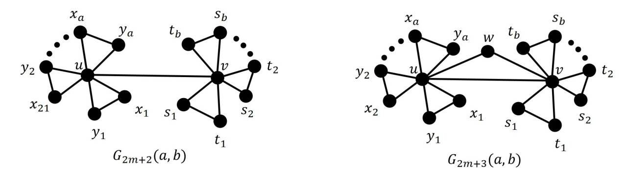
Proposition 4.1. Let \(G_{2m+3}(a,b)\) and \(G_{2m+2}(a,b)\) be the graphs defined above.
(i) Suppose that \(n=2m+3\), and let \(a,b\ge 1\) with \(a+b=m\). Then \[\mathrm{Spec}(\mathcal{L}(G_{2m+3}(a,b))) = \left\{ 0^{(1)}, \left(\frac12\right)^{(a+b-2)}, \left(\frac32\right)^{(a+b+2)}, \lambda_-^{(1)}, \lambda_+^{(1)} \right\},\] where \[\lambda_{\pm} = \frac12 \pm \frac12 \sqrt{\frac{ab}{(a+1)(b+1)}}.\]
(ii) Suppose that \(n=2m+2\), and let \(a,b\ge 1\) with \(a+b=m\). Then \[\mathrm{Spec}(\mathcal{L}(G_{2m+2}(a,b))) = \left\{ 0^{(1)}, \left(\frac12\right)^{(a+b-2)}, \left(\frac32\right)^{(a+b)}, \lambda_1^{(1)}, \lambda_2^{(1)}, \lambda_3^{(1)} \right\},\] where \(\lambda_i=1-\mu_i\) \((i=1,2,3)\), and \(\mu_1,\mu_2,\mu_3\) are the three roots of \[4(2a+1)(2b+1)\mu^3-(12ab+2a+2b+3)\mu+(1-4ab)=0.\]
Proof. We first determine the spectrum of the normalized adjacency matrix \(S\).
Let \(u\) and \(v\) be the two vertices of degree greater than \(2\), and write \(d_u=d(u)\) and \(d_v=d(v)\). For \(1\le i\le a\), let \(x_i,y_i\) be the two non-central vertices on the \(i\)th triangle attached to \(u\); for \(1\le j\le b\), let \(s_j,t_j\) be the two non-central vertices on the \(j\)th triangle attached to \(v\). In the odd case \(G_{2m+3}(a,b)\), let \(w\) be the common neighbor of \(u\) and \(v\).
For \(1\le i\le a\) and \(1\le j\le b\), define \(\mathbf{p}_i=\mathbf{e}_{x_i}-\mathbf{e}_{y_i}, \mathbf{q}_j=\mathbf{e}_{s_j}-\mathbf{e}_{t_j}.\) Since \[S\mathbf{e}_{x_i}=\frac12\mathbf{e}_{y_i} +\frac{1}{\sqrt{2d_u}}\mathbf{e}_u,\qquad S\mathbf{e}_{y_i}=\frac12\mathbf{e}_{x_i} +\frac{1}{\sqrt{2d_u}}\mathbf{e}_u,\] and the same calculation holds for \(s_j,t_j\) with \(v\) in place of \(u\), we get \[S\mathbf{p}_i=-\frac12 \mathbf{p}_i,\qquad S\mathbf{q}_j=-\frac12 \mathbf{q}_j.\]
Thus \[W_-=\operatorname{span}\{\mathbf{p}_1,\ldots,\mathbf{p}_a, \mathbf{q}_1,\ldots,\mathbf{q}_b\},\] is \(S\)-invariant, \(S|_{W_-}=-\frac12 I\), and \(\dim W_-=a+b\). Hence \(-1/2\) is an eigenvalue of \(S\) with multiplicity at least \(a+b\).
Next, let \(\boldsymbol{\alpha}_i=\mathbf{e}_{x_i}+\mathbf{e}_{y_i}\quad (1\le i\le a), \boldsymbol{\beta}_j=\mathbf{e}_{s_j}+\mathbf{e}_{t_j}\quad (1\le j\le b),\) and set \[W_u=\left\{\sum_{i=1}^a c_i\boldsymbol{\alpha}_i:\ \sum_{i=1}^a c_i=0\right\},\qquad W_v=\left\{\sum_{j=1}^b d_j\boldsymbol{\beta}_j:\ \sum_{j=1}^b d_j=0\right\}.\]
For each \(i\) and \(j\), \[S\boldsymbol{\alpha}_i =\frac12\boldsymbol{\alpha}_i+\frac{2}{\sqrt{2d_u}}\mathbf{e}_u, \qquad S\boldsymbol{\beta}_j =\frac12\boldsymbol{\beta}_j+\frac{2}{\sqrt{2d_v}}\mathbf{e}_v.\]
Hence, for every \(\mathbf{x}\in W_u\oplus W_v\), the coefficients of the \(\mathbf{e}_u\) and \(\mathbf{e}_v\) terms vanish, and \[S\mathbf{x}=\frac12\mathbf{x}.\]
Therefore \(W_u\oplus W_v\) is \(S\)-invariant, and \[\dim(W_u\oplus W_v)=(a-1)+(b-1)=a+b-2.\]
Therefore \(1/2\) is an eigenvalue of \(S\) with multiplicity at least \(a+b-2\).
It remains to determine the remaining eigenvalues.
Case 1. \(n=2m+3\).
In this case, \(d(u)=2a+2=:d_u, d(v)=2b+2=:d_v, d(w)=2,\) and every vertex in \[U=\{x_i,y_i:1\le i\le a\},\qquad V=\{s_j,t_j:1\le j\le b\},\] has degree \(2\). Let \[\mathcal U_\pi=\operatorname{span}\{\mathbf e_u,\mathbf e_v,\mathbf e_w, \mathbf 1_U,\mathbf 1_V\}.\]
Then \[\mathbb R^{V(G_{2m+3}(a,b))} =W_-\oplus W_u\oplus W_v\oplus \mathcal U_\pi,\] is an orthogonal direct sum. Indeed, for all admissible indices, \[\langle \mathbf p_i,\boldsymbol{\alpha}_k\rangle=0,\qquad \langle \mathbf q_j,\boldsymbol{\beta}_\ell\rangle=0,\] and all other inner products between a difference vector from \(W_-\) and a sum vector from \(W_u\oplus W_v\) vanish by disjoint support. Moreover, \[\langle \mathbf p_i,\mathbf 1_U\rangle=0,\qquad \langle \mathbf q_j,\mathbf 1_V\rangle=0,\] and \(W_-\) is orthogonal to \(\mathbf e_u,\mathbf e_v,\mathbf e_w\). If \(\mathbf x=\sum_i c_i\boldsymbol{\alpha}_i\in W_u\), then \[\langle \mathbf x,\mathbf 1_U\rangle=2\sum_i c_i=0,\] and \(\mathbf x\) is orthogonal to \(\mathbf e_u,\mathbf e_v,\mathbf e_w\) and \(\mathbf 1_V\); the same argument applies to \(W_v\). Hence the four subspaces above are mutually orthogonal. Since \[\dim W_-+\dim W_u+\dim W_v+\dim \mathcal U_\pi =(a+b)+(a-1)+(b-1)+5=2a+2b+3,\] their orthogonal sum is the whole space \(\mathbb R^{V(G_{2m+3}(a,b))}\). Thus it remains only to determine the action of \(S\) on the cell-constant subspace \(\mathcal U_\pi\).
Consider the partition \[C_1=\{u\},\quad C_2=\{v\},\quad C_3=\{w\},\quad C_4=U,\quad C_5=V.\]
This is an equitable partition of \(S\). Let \(Q\) be the corresponding quotient matrix. Then \[Q= \begin{pmatrix} 0 & \dfrac{1}{\sqrt{d_ud_v}} & \dfrac{1}{\sqrt{2d_u}} & \dfrac{2a}{\sqrt{2d_u}} & 0\\[1.2ex] \dfrac{1}{\sqrt{d_ud_v}} & 0 & \dfrac{1}{\sqrt{2d_v}} & 0 & \dfrac{2b}{\sqrt{2d_v}}\\[1.2ex] \dfrac{1}{\sqrt{2d_u}} & \dfrac{1}{\sqrt{2d_v}} & 0 & 0 & 0\\[1.2ex] \dfrac{1}{\sqrt{2d_u}} & 0 & 0 & \dfrac12 & 0\\[1.2ex] 0 & \dfrac{1}{\sqrt{2d_v}} & 0 & 0 & \dfrac12 \end{pmatrix}.\]
Let \(\Delta=\operatorname{diag}(1,1,1,2a,2b)\). Then \(Q\) is similar to the symmetric matrix \[B=\Delta^{1/2}Q\Delta^{-1/2}= \begin{pmatrix} 0 & \dfrac{1}{\sqrt{d_ud_v}} & \dfrac{1}{\sqrt{2d_u}} & \sqrt{\dfrac{a}{d_u}} & 0\\[1.2ex] \dfrac{1}{\sqrt{d_ud_v}} & 0 & \dfrac{1}{\sqrt{2d_v}} & 0 & \sqrt{\dfrac{b}{d_v}}\\[1.2ex] \dfrac{1}{\sqrt{2d_u}} & \dfrac{1}{\sqrt{2d_v}} & 0 & 0 & 0\\[1.2ex] \sqrt{\dfrac{a}{d_u}} & 0 & 0 & \dfrac12 & 0\\[1.2ex] 0 & \sqrt{\dfrac{b}{d_v}} & 0 & 0 & \dfrac12 \end{pmatrix}.\]
We now compute its characteristic polynomial. Set \[\eta=\mu-\frac12.\]
For \(\mu\ne\frac12\), applying Lemma 2.2 to the lower-right diagonal block \(\eta I_2\) of \(\mu I-B\) gives \[\begin{aligned} \det(\mu I-B) &=\eta^2 \det \begin{pmatrix} \mu-\dfrac{a}{d_u\eta} & -\dfrac{1}{\sqrt{d_ud_v}} & -\dfrac{1}{\sqrt{2d_u}}\\[3mm] -\dfrac{1}{\sqrt{d_ud_v}} & \mu-\dfrac{b}{d_v\eta} & -\dfrac{1}{\sqrt{2d_v}}\\[3mm] -\dfrac{1}{\sqrt{2d_u}} & -\dfrac{1}{\sqrt{2d_v}} & \mu \end{pmatrix} \\ &=\eta^2\Biggl[ \mu\left(\mu-\frac{a}{d_u\eta}\right) \left(\mu-\frac{b}{d_v\eta}\right) -\frac{1}{2d_v}\left(\mu-\frac{a}{d_u\eta}\right) \\ &\hspace{5mm} -\frac{1}{2d_u}\left(\mu-\frac{b}{d_v\eta}\right) -\frac{\mu+1}{d_ud_v} \Biggr]. \end{aligned}\]
Substituting \(d_u=2a+2\), \(d_v=2b+2\), and \(\eta=\mu-\frac12\), and simplifying, we obtain \[\det(\mu I-B) = (\mu-1)\Bigl(\mu+\frac12\Bigr)^2 \Bigl(\mu^2-\mu+\frac{a+b+1}{4(a+1)(b+1)}\Bigr).\]
Since both sides are polynomials in \(\mu\), the identity also holds for \(\mu=\frac12\). Hence the eigenvalues of \(Q\) are \[1,\quad -\frac12\ \text{(with multiplicity $2$)},\quad \mu_\pm=\frac12\pm \frac12\sqrt{\frac{ab}{(a+1)(b+1)}}.\]
By Lemma 2.4, we have \(\mathrm{Spec}(Q)\subseteq \mathrm{Spec}(S).\) Since \((a+b)+(a+b-2)+5=2a+2b+3=|V(G_{2m+3}(a,b))|,\) the above eigenvalues account for the whole spectrum of \(S\). Therefore \[\mathrm{Spec}(S(G_{2m+3}(a,b)))= \Bigl\{1^{(1)},\, \Bigl(\frac12\Bigr)^{(a+b-2)},\, \Bigl(-\frac12\Bigr)^{(a+b+2)},\, \mu_-^{(1)},\,\mu_+^{(1)}\Bigr\}.\]
Since \(\mathcal L=I-S\), we obtain \[\mathrm{Spec}(\mathcal L(G_{2m+3}(a,b)))= \Bigl\{0^{(1)},\, \Bigl(\frac12\Bigr)^{(a+b-2)},\, \Bigl(\frac32\Bigr)^{(a+b+2)},\, \lambda_-^{(1)},\,\lambda_+^{(1)}\Bigr\},\] where \(\lambda_\pm=1-\mu_\mp =\frac12\pm \frac12\sqrt{\frac{ab}{(a+1)(b+1)}}.\)
Case 2. \(n=2m+2\).
In this case, \(d(u)=2a+1=:d_u, d(v)=2b+1=:d_v,\) and every vertex in \[U=\{x_i,y_i:1\le i\le a\},\qquad V=\{s_j,t_j:1\le j\le b\}\] has degree \(2\). Let \[\mathcal U_\pi=\operatorname{span}\{\mathbf e_u,\mathbf e_v,\mathbf 1_U,\mathbf 1_V\}.\]
Then \[\mathbb R^{V(G_{2m+2}(a,b))} =W_-\oplus W_u\oplus W_v\oplus \mathcal U_\pi,\] is an orthogonal direct sum. The orthogonality of \(W_-\), \(W_u\), and \(W_v\) is the same as in the odd case. Also \(W_-\) is orthogonal to \(\mathcal U_\pi\), because each difference vector has coordinate sum zero on the corresponding pair and has no support on \(u\) or \(v\). If \(\mathbf x=\sum_i c_i\boldsymbol{\alpha}_i\in W_u\), then \[\langle \mathbf x,\mathbf 1_U\rangle=2\sum_i c_i=0,\] and \(\mathbf x\) is orthogonal to \(\mathbf e_u,\mathbf e_v\) and \(\mathbf 1_V\); similarly \(W_v\perp\mathcal U_\pi\). Since \[\dim W_-+\dim W_u+\dim W_v+\dim \mathcal U_\pi =(a+b)+(a-1)+(b-1)+4=2a+2b+2,\] their orthogonal sum is the whole space \(\mathbb R^{V(G_{2m+2}(a,b))}\). Thus the remaining eigenvalues are obtained from the action of \(S\) on \(\mathcal U_\pi\).
Consider the partition \[C_1=\{u\},\quad C_2=\{v\},\quad C_3=U,\quad C_4=V.\]
This is an equitable partition of \(S\). Let \(Q\) be the corresponding quotient matrix. Then \[Q= \begin{pmatrix} 0 & \dfrac{1}{\sqrt{d_ud_v}} & \dfrac{2a}{\sqrt{2d_u}} & 0\\[1.2ex] \dfrac{1}{\sqrt{d_ud_v}} & 0 & 0 & \dfrac{2b}{\sqrt{2d_v}}\\[1.2ex] \dfrac{1}{\sqrt{2d_u}} & 0 & \dfrac12 & 0\\[1.2ex] 0 & \dfrac{1}{\sqrt{2d_v}} & 0 & \dfrac12 \end{pmatrix}.\]
Let \(\Delta=\operatorname{diag}(1,1,2a,2b)\). Then \(Q\) is similar to the symmetric matrix \[B=\Delta^{1/2}Q\Delta^{-1/2}= \begin{pmatrix} 0 & \dfrac{1}{\sqrt{d_ud_v}} & \sqrt{\dfrac{a}{d_u}} & 0\\[1.2ex] \dfrac{1}{\sqrt{d_ud_v}} & 0 & 0 & \sqrt{\dfrac{b}{d_v}}\\[1.2ex] \sqrt{\dfrac{a}{d_u}} & 0 & \dfrac12 & 0\\[1.2ex] 0 & \sqrt{\dfrac{b}{d_v}} & 0 & \dfrac12 \end{pmatrix}.\]
We compute the determinant in detail. Again set \[\eta=\mu-\frac12.\]
For \(\mu\ne\frac12\), applying Lemma 2.2 to the lower-right diagonal block \(\eta I_2\) of \(\mu I-B\) yields \[\begin{aligned} \det(\mu I-B) &=\eta^2 \det \begin{pmatrix} \mu-\dfrac{a}{d_u\eta} & -\dfrac{1}{\sqrt{d_ud_v}}\\[3mm] -\dfrac{1}{\sqrt{d_ud_v}} & \mu-\dfrac{b}{d_v\eta} \end{pmatrix} \\ &=\eta^2\left[ \left(\mu-\frac{a}{d_u\eta}\right) \left(\mu-\frac{b}{d_v\eta}\right) -\frac{1}{d_ud_v} \right] \\ &=\frac{1}{d_ud_v} \left[ (d_u\mu\eta-a)(d_v\mu\eta-b)-\eta^2 \right]. \end{aligned}\]
Since \(d_u=2a+1\) and \(d_v=2b+1\), we have \[d_ud_v=4ab+2a+2b+1,\qquad d_ub+d_va=4ab+a+b.\]
Therefore \[\begin{aligned} \det(\mu I-B) &=\frac{1}{(2a+1)(2b+1)} \Bigl[ (2a+1)(2b+1)\mu^2\left(\mu-\frac12\right)^2 \\ &\quad -(4ab+a+b)\mu\left(\mu-\frac12\right) +ab-\left(\mu-\frac12\right)^2 \Bigr] \\ &=\frac{\mu-1}{4(2a+1)(2b+1)} \Bigl( 4(2a+1)(2b+1)\mu^3 \\ &\quad -(12ab+2a+2b+3)\mu+(1-4ab) \Bigr). \end{aligned}\]
Again, since both sides are polynomials, the identity holds for all \(\mu\). Hence the eigenvalues of \(Q\) are \[1,\ \mu_1,\ \mu_2,\ \mu_3,\] where \(\mu_1,\mu_2,\mu_3\) are the three roots of \[4(2a+1)(2b+1)\mu^3-(12ab+2a+2b+3)\mu+(1-4ab)=0.\]
Again, by Lemma 2.4, \(\mathrm{Spec}(Q)\subseteq \mathrm{Spec}(S).\) Since \((a+b)+(a+b-2)+4=2a+2b+2=|V(G_{2m+2}(a,b))|,\) these eigenvalues account for all eigenvalues of \(S\). Thus \[\mathrm{Spec}(S(G_{2m+2}(a,b)))= \Bigl\{1^{(1)},\, \Bigl(\frac12\Bigr)^{(a+b-2)},\, \Bigl(-\frac12\Bigr)^{(a+b)},\, \mu_1^{(1)},\,\mu_2^{(1)},\,\mu_3^{(1)}\Bigr\}.\]
Therefore \[\mathrm{Spec}(\mathcal{L}(G_{2m+2}(a,b)))= \Bigl\{0^{(1)},\, \Bigl(\frac12\Bigr)^{(a+b-2)},\, \Bigl(\frac32\Bigr)^{(a+b)},\, \lambda_1^{(1)},\,\lambda_2^{(1)},\,\lambda_3^{(1)}\Bigr\},\] where \(\lambda_i=1-\mu_i\) for \(i=1,2,3\). \(\square\)
Lemma 4.2. Let \(n \ge 6\) be even, and let \(G_{2m+2}(a,b)\) be the graph defined above. Then \[\rho(\mathcal{L}(G_{2m+2}(a,b)))<\frac32+\frac{1}{n+1}.\]
Proof. By Proposition 4.1(ii), the eigenvalues of \(S\) different from \(-1/2\) are precisely the three roots of \[P(\mu)=4(2a+1)(2b+1)\mu^3-(12ab+2a+2b+3)\mu+(1-4ab),\] where \(a,b\ge 1\) and \(n=2a+2b+2\).
Since \(P\!\left(-\frac12\right)=2>0\) and \(P(\mu)\to -\infty (\mu\to -\infty),\) the polynomial \(P\) has a root in \((-\infty,-1/2)\). Moreover, \[P'(\mu)=12(2a+1)(2b+1)\mu^2-(12ab+2a+2b+3).\]
Thus, for \(\mu\le -1/2\), \[P'(\mu)\ge 3(2a+1)(2b+1)-(12ab+2a+2b+3)=4(a+b)>0.\]
Hence \(P\) is strictly increasing on \((-\infty,-1/2]\), and therefore it has a unique root \[\mu_1\in(-\infty,-1/2).\]
Since the other eigenvalue \(-1/2\) has multiplicity \(a+b\), it follows that \(\mu_{\min}(S)=\mu_1.\)
Set \(\mu_0=-\frac12-\frac{1}{n+1}.\) It suffices to prove \(\mu_1>\mu_0\), because then \[\rho(\mathcal{L}(G_{2m+2}(a,b)))=1-\mu_{\min}(S)<1-\mu_0=\frac32+\frac{1}{n+1}.\]
Now \[n+1=2(a+b)+3,\] and substituting \(\mu_0=-\frac12-\frac1{n+1}\) into \(P\), we obtain \[P(\mu_0)= \frac{8\bigl(-6a^2b-6ab^2-11ab+2a+2b+4\bigr)}{(2a+2b+3)^3}.\]
Let \(s=a+b\). Since \(a,b\ge 1\), we have \(ab\ge a+b-1=s-1.\) Therefore \[\begin{aligned} -6a^2b-6ab^2-11ab+2a+2b+4=&-ab(6s+11)+2s+4\\ \le& -(s-1)(6s+11)+2s+4\\ =&-6s^2-3s+15<0, \end{aligned}\] because \(s\ge 2\). Hence \(P(\mu_0)<0<P\!\left(-\frac12\right).\) Since \(P\) is strictly increasing on \((-\infty,-1/2]\), its unique root \(\mu_1\) in \((-\infty,-1/2)\) satisfies \(\mu_0<\mu_1<-\frac12.\) Thus \(\mu_{\min}(S)=\mu_1>\mu_0,\) and consequently \[\rho(\mathcal{L}(G_{2m+2}(a,b)))=1-\mu_{\min}(S) <1-\mu_0 =\frac32+\frac{1}{n+1}.\]
This completes the proof. \(\square\)
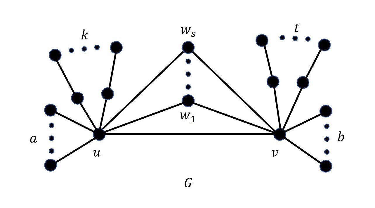
Lemma 4.3. Let \(G \in \mathcal{G}_n\) be a non-bipartite graph. Then the spectral radius of its normalized Laplacian matrix satisfies \(\rho(\mathcal{L}(G)) \ge \frac{3}{2}.\)
Proof. We distinguish two cases.
Case 1. There exists an edge \(xy\in E(G)\) such that \(d(x)=d(y)=2\).
Define \(\mathbf{g}\) on \(V(G)\) by \[g(x)=1,\qquad g(y)=-1,\qquad g(z)=0 \ \text{for all } z\in V(G)\setminus \{x,y\}.\]
Then \[\sum_{ij\in E(G)}(g_i-g_j)^2 =(1-(-1))^2+(1-0)^2+(-1-0)^2=6,\] and \[\sum_{i\in V(G)}d(i) g_i^2 =2\cdot 1^2+2\cdot (-1)^2=4.\]
Hence by Eq. (3) \[\rho(\mathcal L(G))\ge \frac{6}{4}=\frac32.\]
Case 2. There is no edge \(xy\in E(G)\) such that \(d(x)=d(y)=2\).
Since \(G\in\mathcal G_n\), the graph \(G\) has the form shown in Figure 3, where \(a,b\ge 0\), \(s\ge 0\), and \(k,t\ge 0\). Here \(w_1,\dots,w_s\) are the common neighbors of \(u\) and \(v\) of degree \(2\), there are \(a\) leaves adjacent to \(u\), \(b\) leaves adjacent to \(v\), and \(k\) pendant paths of length \(2\) attached to \(u\), \(t\) pendant paths of length \(2\) attached to \(v\). Moreover, \(e\in\{0,1\}\) indicates whether \(uv\in E(G)\).
Since \(G\) is non-bipartite, it contains an odd cycle. Under the assumption of Case 2, this forces \(e=1\) and \(s\ge 1\).
Now define \(\mathbf{g}\) on \(V(G)\) by \[g(u)=-1,\qquad g(x)=1 \ \text{for all } x\in N(u)\setminus \{v\},\qquad g(z)=0 \ \text{for all remaining vertices } z.\]
Then \[\sum_{ij\in E(G)}(g_i-g_j)^2=4a+5s+5k+1,\] and \[\sum_{i\in V(G)}d(i) g_i^2=2a+3s+3k+1.\]
Therefore by Eq. (3) \[\rho(\mathcal L(G)) \ge \frac{4a+5s+5k+1}{2a+3s+3k+1}.\]
It remains to verify that \(\frac{4a+5s+5k+1}{2a+3s+3k+1}\ge \frac32,\) is equivalent to \(2a+s+k-1\ge 0.\) Since \(a\ge 0\), \(k\ge 0\), and \(s\ge 1\), the above inequality holds. Hence \(\rho(\mathcal L(G))\ge \frac32.\)
Combining the two cases, we conclude that \(\rho(\mathcal L(G))\ge \frac32.\) \(\square\)
Lemma 4.4. Let \(G\) be an extremal graph in \(\mathcal{G}_n\), and let \(u\) and \(v\) be the two vertices of \(G\) whose degrees are greater than \(2\). Then \(G\) contains no \(u\)–\(v\) path of length \(3\).
Proof. Suppose, to the contrary, that \(G\) contains a \(u\)–\(v\) path of length \(3\), denoted by \(u-x-y-v\). Since \(u\) and \(v\) are the only vertices of degree greater than \(2\), we have \(d(x)=d(y)=2.\)
Let \(W=\{u,x,y,v\}.\) Set \[\alpha=\frac{1}{\sqrt{d(u)d(x)}}=\frac{1}{\sqrt{2d(u)}}, \qquad \gamma=\frac{1}{\sqrt{d(v)d(y)}}=\frac{1}{\sqrt{2d(v)}},\] and \[\varepsilon= \begin{cases} \dfrac{1}{\sqrt{d(u)d(v)}}, & uv\in E(G),\\[2mm] 0, & uv\notin E(G). \end{cases}\]
With respect to the vertex order \(u,x,y,v\), the principal submatrix of \(S\) indexed by \(W\) is \[S[W]= \begin{pmatrix} 0 & \alpha & 0 & \varepsilon\\ \alpha & 0 & \frac12 & 0\\ 0 & \frac12 & 0 & \gamma\\ \varepsilon & 0 & \gamma & 0 \end{pmatrix},\] which includes the possible additional entries corresponding to the edge \(uv\).
Consider the vector \[\mathbf{z}=(2\alpha,-1,1,-2\gamma)^T.\]
Using the nonzero entries of \(S[W]\), we get \[\begin{aligned} \mathbf{z}^TS[W]\mathbf{z} &=2\alpha(2\alpha)(-1) +2\cdot\frac12(-1)(1) +2\gamma(1)(-2\gamma) +2\varepsilon(2\alpha)(-2\gamma)\\ &=-(1+4\alpha^2+4\gamma^2+8\alpha\gamma\varepsilon), \end{aligned}\] and \[\mathbf{z}^T\mathbf{z} =(2\alpha)^2+(-1)^2+1^2+(-2\gamma)^2 =2+4\alpha^2+4\gamma^2.\]
Since \(\varepsilon\ge 0,\) we have \[\frac{\mathbf{z}^TS[W]\mathbf{z}}{\mathbf{z}^T\mathbf{z}} = -\frac{1+4\alpha^2+4\gamma^2+8\alpha\gamma\varepsilon} {2+4\alpha^2+4\gamma^2} \le -\frac{1+4\alpha^2+4\gamma^2}{2+4\alpha^2+4\gamma^2} <-\frac12.\]
Therefore, by the Rayleigh–Ritz principle, \[\mu_{\min}(S[W]) \le -\frac{1+4\alpha^2+4\gamma^2+8\alpha\gamma\varepsilon} {2+4\alpha^2+4\gamma^2} <-\frac12.\]
By Lemma 2.1, \[\mu_{\min}(S)\le \mu_{\min}(S[W]) \le -\frac{1+4\alpha^2+4\gamma^2+8\alpha\gamma\varepsilon} {2+4\alpha^2+4\gamma^2}.\]
Since \(\mathcal L(G)=I-S\), it follows that \[\rho(\mathcal L(G))=1-\mu_{\min}(S) \ge 1+\frac{1+4\alpha^2+4\gamma^2+8\alpha\gamma\varepsilon} {2+4\alpha^2+4\gamma^2} \ge 1+\frac{1+4\alpha^2+4\gamma^2}{2+4\alpha^2+4\gamma^2}.\]
Set \(s=\alpha^2+\gamma^2.\) \[\rho(\mathcal L(G)) \ge 1+\frac{1+4s}{2+4s} = \frac32+\frac{s}{1+2s}.\]
Moreover, since \(d(x)=d(y)=2\), the vertex \(x\) is not adjacent to \(v\) and the vertex \(y\) is not adjacent to \(u\). Hence \(d(u)\le n-2\) and \(d(v)\le n-2\). It follows that \[s=\frac{1}{2d(u)}+\frac{1}{2d(v)} \ge \frac{1}{2(n-2)}+\frac{1}{2(n-2)} =\frac{1}{n-2}.\]
As the function \(f(t)=\frac{t}{1+2t}\) is strictly increasing on \((0,\infty)\), we obtain \[\rho(\mathcal L(G)) \ge \frac32+\frac{1/(n-2)}{1+2/(n-2)} = \frac32+\frac{1}{n} > \frac32+\frac{1}{n+1}.\]
If \(n\) is odd, then by Proposition 4.1(i), \(\rho(\mathcal L(G_{2m+3}(a,b)))=\frac32.\) If \(n\) is even, then by Lemma 4.2, \(\rho(\mathcal{L}(G_{2m+2}(a,b)))<\frac32+\frac{1}{n+1}.\) In either case, the inequality above contradicts the extremality of \(G\). Therefore, \(G\) contains no \(u\)–\(v\) path of length \(3\). \(\square\)
Lemma 4.5. Let G be an extremal graph in \(\mathcal{G}_n\), and let \(u\) and \(v\) be the two vertices of \(G\) whose degrees are greater than \(2\). If \(x\) is a pendant vertex of G, then \(x\) is adjacent to either \(u\) or \(v\).
Proof. Suppose, to the contrary, that there exists a pendant vertex \(x\) which is adjacent to neither u nor v. Let y be the unique neighbor of \(x\). Since \(y \neq u,v\) and \(u,v\) are the only vertices of G whose degrees are greater than \(2\), we have \(d(y)\le 2\). On the other hand, as \(G\) is connected and \(x\) is pendant vertex, the vertex \(y\) has a neighbor other than \(x\). Hence \(d(y)=2\).
Now define \(\mathbf{f}\in \mathbb{R}^{V(G)}\) by \[f(w)= \begin{cases} 1, & w=x,\\ -1, & w=y,\\ 0, & \text{otherwise}. \end{cases}\]
Then \(\mathbf{f}\neq 0\), and since \(d(x)=1, d(y)=2\), and \(xy\in E(G)\), by Eq. (2), we have \[\mu_{\min}(S)\le \frac{\mathbf{f}^{T}S\mathbf{f}}{\mathbf{f}^{T}\mathbf{f}} = \frac{2S_{xy}f(x)f(y)}{2} = -\frac{1}{\sqrt{d(x)d(y)}} = -\frac{\sqrt{2}}{2}.\]
Therefore, by Eq. (1), \[\rho(\mathcal{L}(G))=1-\mu_{\min}(S)\ge 1+\frac{\sqrt{2}}{2}.\]
If n is odd, then by Proposition 4.1(i), \(\rho(\mathcal{L}(G_{2m+3}(a,b)))=\frac32<1+\frac{\sqrt{2}}{2}.\) If n is even, then by Lemma 4.2, \(\rho(\mathcal{L}(G_{2m+2}(a,b)))<\frac32+\frac{1}{n+1}<1+\frac{\sqrt{2}}{2},\) since \(n\ge 6\). In either case, we obtain \[\rho(\mathcal{L}(G))>\rho(\mathcal{L}(G_n(a,b))),\] contradicting the extremality of \(G\). Hence every pendant vertex of \(G\) must be adjacent to either \(u\) or \(v\). \(\square\)
Lemma 4.6. Let \(G\) be an extremal graph in \(\mathcal{G}_n\), and let \(u\) and \(v\) be the two vertices of \(G\) whose degrees are greater than \(2\). If \(z\) is a vertex of degree \(2\) with \(N(z)=\{x,y\}\), then \(xy\in E(G)\). Moreover, the triangle containing \(z\) contains at least one of \(u\) and \(v\).
Proof. Suppose, to the contrary, that there exists a vertex \(z\) of degree \(2\) which does not lie in any triangle. Let \[W=\{w\in V(G): d(w)=2\},\] and let \(H\) be the connected component of \(G[W]\) containing \(z\).
Since every vertex of \(H\) has degree at most \(2\) in \(H\), the graph \(H\) is either a path or a cycle. It cannot be a cycle, for otherwise every vertex of \(H\) would already have two neighbors in \(H\), and hence no vertex of \(H\) could have a neighbor outside \(H\). Thus \(H\) would be a connected component of \(G\), contrary to the connectedness of \(G\). Therefore \(H\) is a path. Write \[H=p_1p_2\cdots p_r,\] where \(r\ge 1\) and \(z\in V(H)\).
Let \(p\) be an endpoint of \(H\), and let \(q\notin V(H)\) be a neighbor of \(p\). Since \(q\notin W\), we have \(d(q)\neq 2\). If \(d(q)=1\), then \(q\) is a pendant vertex adjacent to \(p\), which is impossible by Lemma 4.5, because every pendant vertex is adjacent to either \(u\) or \(v\), while \(d(p)=2\). Hence \(d(q)>2\), so \(q\in\{u,v\}\). Consequently, every neighbor of an endpoint of \(H\) outside \(H\) belongs to \(\{u,v\}\).
We now distinguish three cases.
Case 1. \(r\ge 3\).
Since \(H\) is a connected component of \(G[W]\), there is no edge between nonconsecutive vertices of \(p_1,\dots,p_r\). Hence \(p_1p_2\cdots p_r\) is an induced path in \(G\), and \(d(p_i)=2\) for all \(i\). By Lemma 3.4, \[\rho(\mathcal{L}(G))\ge 1+\cos\frac{\pi}{r+1}\ge 1+\cos\frac{\pi}{4}=1+\frac{\sqrt{2}}{2}.\]
If \(n\) is odd, then Proposition 4.1(i) gives \(\rho(\mathcal{L}(G_{2m+3}(a,b)))=\frac32\). If \(n\) is even, then Lemma 4.2 gives \[\rho(\mathcal{L}(G_{2m+2}(a,b)))<\frac32+\frac{1}{n+1}<1+\frac{\sqrt{2}}{2},\] because \(n\ge 6\). In either case, this contradicts the extremality of \(G\).
Case 2. \(r=2\).
Let \(H=p_1p_2\). Let \(a\) and \(b\) be the neighbors of \(p_1\) and \(p_2\) outside \(H\), respectively. By the previous paragraph, \(a,b\in\{u,v\}\). If \(a=b\), then \(ap_1p_2a\) is a triangle, contrary to the choice of \(z\). Hence \(a\neq b\), and therefore \(\{a,b\}=\{u,v\}\). Thus \(u-p_1-p_2-v\) is a \(u\)–\(v\) path of length \(3\), contradicting Lemma 4.4.
Case 3. \(r=1\).
Then \(H=\{z\}\). Both neighbors of \(z\) lie outside \(W\), and by the above argument they belong to \(\{u,v\}\). Since \(G\) is simple, these two neighbors are distinct, so \[N(z)=\{u,v\}.\]
Because \(z\) does not lie in a triangle, we must have \(uv\notin E(G)\).
We now justify that this local conclusion determines the structure of all components of \(G[W]\). Let \(H’\) be an arbitrary connected component of \(G[W]\). As above, \(H’\) cannot be a cycle; otherwise \(H’\) would have no edge to \(V(G)\setminus W\), and hence would be a connected component of \(G\). Thus \[H’=q_1q_2\cdots q_t,\] is a path. If \(p\) is an endpoint of \(H’\) and \(r\notin V(H’)\) is the other neighbor of \(p\), then \(r\notin W\). The vertex \(r\) cannot be pendant, because Lemma 4.5 says that every pendant vertex is adjacent to \(u\) or \(v\), whereas \(p\) has degree \(2\). Hence \(d(r)>2\), and so \(r\in\{u,v\}\). Thus every component of \(G[W]\) is a path whose endpoints are attached only to vertices in \(\{u,v\}\).
The case \(t\ge 3\) is impossible by the same induced-path argument used in Case 1. If \(t=2\), say \(H’=q_1q_2\), then the endpoint attachments cannot be different vertices of \(\{u,v\}\), for otherwise \(u-q_1-q_2-v\) or \(v-q_1-q_2-u\) would be a \(u\)–\(v\) path of length \(3\), contradicting Lemma 4.4. Hence both endpoints of \(H’\) are attached to the same one of \(u\) and \(v\), and \(H’\) is exactly the pair of non-central vertices in a triangle attached to \(u\) or to \(v\). If \(t=1\), then the unique vertex of \(H’\) has both its neighbors outside \(W\); by the preceding paragraph these two neighbors are precisely \(u\) and \(v\). Thus every one-vertex component of \(G[W]\) is a common neighbor of \(u\) and \(v\).
There are no further edges among the vertices just described. Indeed, an edge between two distinct components of \(G[W]\) would merge them into one component; an additional edge incident with a degree-\(2\) vertex would contradict its degree; and every pendant vertex has only its unique incident edge. The only possible additional edge among the attachment vertices is \(uv\), but \(uv\notin E(G)\) in the present case. By Lemma 4.5, every pendant vertex of \(G\) is adjacent to \(u\) or \(v\). Consequently, \(G\) has the following structure: there are \(s\ge 1\) common neighbors of \(u\) and \(v\), \(a\ge 0\) triangles attached to \(u\), \(b\ge 0\) triangles attached to \(v\), and \(m\ge 0\) pendant vertices adjacent to \(u\) or \(v\), with \(uv\notin E(G)\). Therefore \[n=2+s+2(a+b)+m.\]
Define \(\mathbf{g}\in \mathbb{R}^{V(G)}\) by \[g(w)= \begin{cases} 1, & w\in\{u,v\},\\ -1, & w \text{ is a common neighbor of }u\text{ and }v,\\ -\frac12, & w \text{ is a degree-}2\text{ vertex in a triangle attached to }u\text{ or }v,\\ -1, & w \text{ is a pendant vertex adjacent to }u\text{ or }v,\\ 0, & \text{otherwise}. \end{cases}\]
By the structure described above and by the definition of \(\mathbf{g}\), the numerator in the Rayleigh quotient (3) is \[\begin{aligned} \sum_{xy\in E(G)}(g(x)-g(y))^2 &=s\bigl[(1+1)^2+(1+1)^2\bigr] +(a+b)\left[2\left(1+\frac12\right)^2+ \left(-\frac12+\frac12\right)^2\right] \\ &\quad +m(1+1)^2 =8s+\frac92(a+b)+4m. \end{aligned}\]
For the denominator, let \(m_u\) and \(m_v\) be the numbers of pendant vertices adjacent to \(u\) and \(v\), respectively. Then we have \[\begin{aligned} m&=m_u+m_v,\\ d(u)+d(v) &=\bigl(s+2a+m_u\bigr)+\bigl(s+2b+m_v\bigr) =2s+2(a+b)+m, \end{aligned}\] and \[\begin{aligned} \sum_{x\in V(G)}d(x)g(x)^2 &=\bigl(d(u)+d(v)\bigr)+2s+(a+b)+m\\ &=\bigl(2s+2(a+b)+m\bigr)+2s+(a+b)+m\\ &=4s+3(a+b)+2m. \end{aligned}\]
Hence, by Eq. (3), \[\rho(\mathcal{L}(G)) \ge \frac{8s+\frac92(a+b)+4m}{4s+3(a+b)+2m} = \frac32+\frac{2s+m}{4s+3(a+b)+2m}.\]
Using \(n=2+s+2(a+b)+m\), we obtain \[4s+3(a+b)+2m=\frac52 s+\frac12 m+\frac32 n-3.\]
Therefore \[\rho(\mathcal{L}(G)) \ge \frac32+\frac{2s+m}{\frac52 s+\frac12 m+\frac32 n-3}.\]
Moreover, \[2(2s+m)(n+1)-\bigl(5s+m+3n-6\bigr) = s(4n-1)+m(2n+1)-3n+6 \ge n+5>0,\] since \(s\ge 1\), \(m\ge 0\), and \(n\ge 6\). Thus \[\frac{2s+m}{\frac52 s+\frac12 m+\frac32 n-3}>\frac{1}{n+1},\] and hence \[\rho(\mathcal{L}(G))>\frac32+\frac{1}{n+1}.\]
If \(n\) is odd, then Proposition 4.1(i) gives \(\rho(\mathcal{L}(G_{2m+3}(a,b)))=\frac32\). If \(n\) is even, then Lemma 4.2 gives \(\rho(\mathcal{L}(G_{2m+2}(a,b)))<\frac32+\frac{1}{n+1}\). In either case, this contradicts the extremality of \(G\).
We have proved that every vertex of degree \(2\) in \(G\) lies in a triangle. Therefore, if \(z\) is a vertex of degree \(2\) and \(N(z)=\{x,y\}\), then the triangle containing \(z\) must use its two neighbors \(x\) and \(y\). Hence \(xy\in E(G).\)
It remains to locate this triangle. Let \(\Delta\) be any triangle containing a degree-\(2\) vertex. If neither \(u\) nor \(v\) belongs to \(\Delta\), then all three vertices of \(\Delta\) have degree at most \(2\). Since each of them already has two neighbors inside \(\Delta\), all three have degree exactly \(2\) in \(G\) and no neighbor outside \(\Delta\). Thus \(\Delta\) would be a connected component of \(G\), contrary to the connectedness of \(G\). Hence every triangle containing a degree-\(2\) vertex contains at least one of \(u\) and \(v\). The proof is complete. \(\square\)
Lemma 4.7. Let \(G\) be an extremal graph in \(\mathcal{G}_n\). Then \(\delta(G)\ge 2.\)
Proof. Suppose, to the contrary, that \(G\) contains a pendant vertex. Let \(u\) and \(v\) be the two vertices of \(G\) whose degrees are greater than \(2\). By Lemma 4.6, every vertex of degree \(2\) lies in a triangle containing \(u\) or \(v\). Hence \(G\) has the following structure: there are \(s\ge 0\) common neighbors of \(u\) and \(v\), \(t\ge 0\) pendant vertices adjacent to \(u\), \(r\ge 0\) pendant vertices adjacent to \(v\), \(a\ge 0\) triangles attached to \(u\), and \(b\ge 0\) triangles attached to \(v\); moreover, possibly \(uv\in E(G)\). Let \(e\in\{0,1\}\) indicate whether \(uv\in E(G)\), that is, \(e=1\) if \(uv\in E(G)\), and \(e=0\) otherwise. Then \(n=2+s+t+r+2a+2b,\) and \[d(u)=e+s+t+2a=:d_u,\qquad d(v)=e+s+r+2b=:d_v.\]
Assume first that \(t\ge 1\), the case \(r\ge 1\) is symmetric. Define \(\mathbf{x}\in \mathbb{R}^{V(G)}\) by \[x(z)= \begin{cases} 1, & z=u,\\[1mm] -\dfrac{2}{\sqrt{d_u}}, & z \text{ is a pendant vertex adjacent to }u,\\[2mm] -\sqrt{\dfrac{2}{d_u}}, & z \in N(u)\cap N(v),\\[2mm] -\dfrac{1}{\sqrt{2d_u}}, & z\in\{x_i,y_i\}\text{ for some triangle }\Delta(u,x_i,y_i)\text{ attached to }u,\\[2mm] 0, & \text{otherwise}. \end{cases}\]
For the vector \(\mathbf{x}\) defined above, its squared norm is \[\begin{aligned} \|\mathbf{x}\|^2 &=1+t\frac{4}{d_u}+s\frac{2}{d_u}+2a\frac{1}{2d_u} \\ &=\frac{d_u+4t+2s+a}{d_u} =\frac{e+3s+3a+5t}{d_u}. \end{aligned}\]
Using \(x(v)=0\), so that the edge \(uv\), if present, gives no term, we also obtain \[\begin{aligned} \mathbf{x}^TS\mathbf{x} &=2\sum_{pq\in E(G)}\frac{x(p)x(q)}{\sqrt{d(p)d(q)}}\\ &=t\left(2\cdot\frac{1(-2/\sqrt{d_u})}{\sqrt{d_u}}\right) +s\left(2\cdot\frac{1(-\sqrt{2/d_u})}{\sqrt{2d_u}}\right)\\ &\quad +2a\left(2\cdot\frac{1(-1/\sqrt{2d_u})}{\sqrt{2d_u}}\right) +a\left(2\cdot\frac{(-1/\sqrt{2d_u})^2}{2}\right)+0\\ &=-\frac{4t+2s+\frac32a}{d_u} =-\frac12\|\mathbf{x}\|^2-\frac{s+3t-e}{2d_u}, \end{aligned}\]
Hence \[\frac{\mathbf{x}^TS\mathbf{x}}{\|\mathbf{x}\|^2} = -\frac12-\frac{s+3t-e}{2(e+3s+3a+5t)}.\]
Therefore \[\mu_{\min}(S)\le -\frac12-\Delta_u, \qquad \Delta_u=\frac{s+3t-e}{2(e+3s+3a+5t)}>0.\]
Here \(\Delta_u\) is positive because \(t\ge1\), \(e\le1\), and \[s+3t-e\ge 3-1=2>0,\qquad e+3s+3a+5t>0.\]
By Eq. (1), we obtain \[\rho(\mathcal{L}(G))\ge \frac32+\Delta_u.\]
Similarly, if \(r\ge 1\), then \[\rho(\mathcal{L}(G))\ge \frac32+\Delta_v, \qquad \Delta_v=\frac{s+3r-e}{2(e+3s+3b+5r)}>0.\]
This is obtained by the same construction with the roles of \(u,t,a\) and \(v,r,b\) interchanged. Hence, whenever \(G\) contains a pendant vertex \[\rho(\mathcal{L}(G)) \ge \frac{3}{2} + \max\{\Delta_u,\Delta_v\}.\]
We now distinguish two cases.
Case 1. \(n\) is odd. By Proposition 4.1(i), \(\rho(\mathcal{L}(G_{2m+3}(a,b)))=\frac32.\) Thus, if \(G\) has pendant vertices, then \[\rho(\mathcal{L}(G))>\frac32=\rho(\mathcal{L}(G_{2m+3}(a,b))).\]
This contradicts the extremality of \(G\).
Case 2. \(n\) is even. We show that \(\rho(\mathcal{L}(G))\ge \frac32+\frac{1}{n+1},\) contradicting Lemma 4.2. We distinguish two subcases.
Subcase 2.1. All pendant vertices are adjacent to the same one of \(u\) and \(v\).
Without loss of generality, assume that \(t\ge 1\) and \(r=0\). Then \(s+t\equiv 0 \pmod 2,\) since \(n=2+s+t+2a+2b\) is even. Moreover, \(d(v)=e+s+2b>2.\)
If \(s=0\), then \(t\) is even, and hence \(t\ge 2\). Also, since \(s=0\) and \(r=0\), connectedness forces \(e=1\), and \(d(v)=1+2b>2\) gives \(b\ge 1\). From \[n=2+t+2a+2b,\] we obtain \[2(1+3a+5t)=3n-4+7t-6b.\]
Hence \[\Delta_u=\frac{3t-1}{3n-4+7t-6b}.\]
To compare this with \(1/(n+1)\), note that the denominator is positive and \[\begin{aligned} (3t-1)(n+1)-(3n-4+7t-6b) &=(6t-8)a+(6t-2)b+3t^2-2t-5 \\ &\ge (6t-2)+3t^2-2t-5 \\ &=3t^2+4t-7>0, \end{aligned}\] where we used \(n=2+t+2a+2b\), \(a\ge0\), \(b\ge1\), and \(t\ge2\). It follows that \[\Delta_u>\frac1{n+1}.\]
Now assume that \(s\ge1\). Let \[N=s+3t-e,\qquad D=2(e+3s+3a+5t),\] so that \(\Delta_u=N/D\). Since \(s+t\) is even and \(s,t\ge1\), either \((s,t)=(1,1)\) or \(s+t\ge4\). Using \[a=\frac{n-2-s-t-2b}{2},\] we have \[D=3n-6+2e+3s+7t-6b.\] If \((s,t)=(1,1)\), then \[N(n+1)-D= \begin{cases} n+6b, & e=0,\\ 6b-3, & e=1. \end{cases}\]
In the second line \(d(v)=1+1+2b>2\), so \(b\ge1\); hence \(N(n+1)-D>0\). If \(s+t\ge4\), then \(N-3=s+3t-e-3>0\), and the expression \[N(n+1)-D,\] can be estimated directly \[\begin{aligned} N(n+1)-D &=(s+3t-e-3)n-2s-4t+6-3e+6b \\ &\ge (s+3t-4)n-2s-4t+3 \\ &\ge 6(s+3t-4)-2s-4t+3 \\ &=4s+14t-21>0. \end{aligned}\]
Here we used \(e\le1\), \(b\ge0\), \(n\ge6\), and the fact that \(s,t\ge1\) with \(s+t\ge4\). Thus \(N(n+1)>D\) in all cases, and so \[\Delta_u>\frac1{n+1}.\]
In either case, \[\rho(\mathcal{L}(G))\ge \frac32+\Delta_u>\frac32+\frac{1}{n+1}.\]
Subcase 2.2. Pendant vertices are adjacent to both \(u\) and \(v\).
Assume that \(t\ge 1, r\ge 1.\) For fixed \(s,e,a\), the function \[f(t) = \frac{s+3t-e}{2(e+3s+3a+5t)},\] is increasing, since its derivative has numerator \[3(e+3s+3a+5t)-5(s+3t-e)=8e+4s+9a\ge0.\]
Therefore \(t\ge1\) implies the following lower bound for \(\Delta_u\). Similarly, using \(r\ge1\) gives the corresponding lower bound for \(\Delta_v\). Then \[\Delta_u\ge \frac{s+3-e}{2(e+3s+3a+5)}, \qquad \Delta_v\ge \frac{s+3-e}{2(e+3s+3b+5)}.\]
Taking the average of these two lower bounds, and using \[\frac{1}{X}+\frac{1}{Y}\ge \frac{4}{X+Y}\qquad (X,Y>0),\] we obtain \[\max\{\Delta_u,\Delta_v\}\ge \frac{\Delta_u+\Delta_v}{2} \ge \frac{s+3-e}{2e+6s+3(a+b)+10}.\]
Since \(n=2+s+t+r+2a+2b\ge 4+s+2a+2b,\) we have \[a+b\le \frac{n-s-4}{2}.\]
Therefore \[\max\{\Delta_u,\Delta_v\} \ge \frac{s+3-e}{2e+6s+\frac32(n-s-4)+10} = \frac{2(s+3-e)}{4e+9s+3n+8}.\]
For even \(n\ge8\), the last expression is decreasing when \(e\) changes from \(0\) to \(1\), and for each fixed \(e\) it is increasing in \(s\). Hence its minimum is attained at \(e=1\) and \(s=0\). Thus \[\max\{\Delta_u,\Delta_v\}\ge \frac{4}{3(n+4)}.\]
If \(n\ge 8\), then \[\frac{4}{3(n+4)}\ge \frac{1}{n+1}.\]
It remains to consider the boundary case \(n=6\), because the preceding estimate uses \(n\ge8\). Then \(6=2+s+t+r+2a+2b,\) and hence \(s+t+r+2a+2b=4.\) Since \(t\ge 1\) and \(r\ge 1\), we have \(a+b\le 1\).
We first show that \(e=1\). Suppose, to the contrary, that \(e=0\). Then, in order for \(G\) to be connected, we must have \(s\ge 1\); otherwise the graph would split into two components, one containing \(u\) and the other containing \(v\). Let \(z\in N(u)\cap N(v)\). Then \(d(z)=2\), and by Lemma 4.6 the vertex \(z\) lies in a triangle containing \(u\) or \(v\). Since \(N(z)=\{u,v\}\), this is possible only if \(uv\in E(G)\), contradicting \(e=0\). Therefore \(e=1\).
Next we claim that \(a=b=0\). Indeed, if \(a+b=1\), then from \[s+t+r+2a+2b=4,\] it follows that \[s+t+r=2.\]
Together with \(t\ge 1\) and \(r\ge 1\), this yields \[s=0,\qquad t=r=1.\]
Since \(a+b=1\), one of \(a,b\) is equal to \(0\). But then one of \[d(u)=1+s+t+2a,\qquad d(v)=1+s+r+2b,\] is equal to \(2\), contradicting the assumption that \(d(u),d(v)>2\). Hence \(a+b=0\), that is, \[a=b=0.\]
Consequently, \[s+t+r=4,\] and \[\Delta_u=\frac{s+3t-1}{2(1+3s+5t)},\qquad \Delta_v=\frac{s+3r-1}{2(1+3s+5r)}.\]
Since \(t\ge 1\) and \(r\ge 1\), we have \[\Delta_u-\frac16 =\frac{3(s+3t-1)-(1+3s+5t)}{6(1+3s+5t)} =\frac{4(t-1)}{6(1+3s+5t)}\ge 0,\] and similarly \[\Delta_v-\frac16 =\frac{3(s+3r-1)-(1+3s+5r)}{6(1+3s+5r)} =\frac{4(r-1)}{6(1+3s+5r)}\ge 0.\]
Therefore \[\max\{\Delta_u,\Delta_v\}\ge \frac16>\frac17=\frac1{n+1}.\]
Hence, in this case, \[\rho(\mathcal{L}(G))\ge \frac32+\max\{\Delta_u,\Delta_v\}> \frac32+\frac1{n+1}.\]
Combining the two subcases, we have \[\rho(\mathcal{L}(G))\ge \frac32+\frac{1}{n+1}.\]
Subcase 2.1 gives a strict inequality. In Subcase 2.2, equality can occur only in the boundary estimate, and the non-strict bound already suffices for the comparison with the even-order candidate below. By Lemma 4.2, \[\rho(\mathcal{L}(G_{2m+2}(a,b)))<\frac32+\frac{1}{n+1},\] again contradicting the extremality of \(G\).
Therefore \(G\) contains no pendant vertex. That is \(\delta(G)\ge 2.\) \(\square\)
Lemma 4.8. Let \(G\) be an extremal graph in \(\mathcal{G}_n\), and let \(u\) and \(v\) be the two vertices of \(G\) whose degrees are greater than \(2\). If every vertex in \(V(G)\setminus\{u,v\}\) has degree \(2\) and lies in a triangle containing \(u\) or \(v\), then \[|N(u)\cap N(v)|\le 1.\]
In particular, \(G\) contains no \(4\)-cycle.
Proof. Set \(s=|N(u)\cap N(v)|.\) We prove that \(s\le 1\). Suppose, to the contrary, that \(s\ge 2\).
Since every common neighbor of \(u\) and \(v\) has degree \(2\) and lies in a triangle containing \(u\) or \(v\), it follows that \(uv\in E(G)\). Let \(U\) be the set of all degree-\(2\) vertices lying in triangles containing \(u\) but not adjacent to \(v\), and let \(V\) be the set of all degree-\(2\) vertices lying in triangles containing \(v\) but not adjacent to \(u\). Then \[|U|=2a,\qquad |V|=2b,\] where \(a,b\ge 0\), and let \[C=N(u)\cap N(v),\qquad |C|=s.\]
Then \[V(G)=\{u,v\}\cup U\cup V\cup C,\] and hence \[n=2+2a+2b+s.\]
Moreover, \[d_u:=d(u)=1+2a+s,\qquad d_v:=d(v)=1+2b+s.\]
Consider the partition \(\pi=\{\{u\},\{v\},U,V,C\},\) this is an equitable partition of \(S\), then the quotient matrix \(Q=(q_{ij})\) is \[Q= \begin{pmatrix} 0 & \dfrac{1}{\sqrt{d_ud_v}} & \dfrac{2a}{\sqrt{2d_u}} & 0 & \dfrac{s}{\sqrt{2d_u}}\\[3mm] \dfrac{1}{\sqrt{d_ud_v}} & 0 & 0 & \dfrac{2b}{\sqrt{2d_v}} & \dfrac{s}{\sqrt{2d_v}}\\[3mm] \dfrac{1}{\sqrt{2d_u}} & 0 & \dfrac12 & 0 & 0\\[3mm] 0 & \dfrac{1}{\sqrt{2d_v}} & 0 & \dfrac12 & 0\\[3mm] \dfrac{1}{\sqrt{2d_u}} & \dfrac{1}{\sqrt{2d_v}} & 0 & 0 & 0 \end{pmatrix}.\]
Let \[D_\pi=\operatorname{diag}\bigl(1,1,\sqrt{2a},\sqrt{2b},\sqrt{s}\bigr),\] again with the zero-size entries deleted. Since \(S\) is symmetric, the quotient row sums satisfy \(|P_i|q_{ij}=|P_j|q_{ji}\), where \(P_i\) denotes the \(i\)-th cell of \(\pi\). Hence \(Q\) is diagonally similar to the symmetric matrix \[B=D_\pi QD_\pi^{-1}= \begin{pmatrix} 0 & \dfrac{1}{\sqrt{d_ud_v}} & \sqrt{\dfrac{a}{d_u}} & 0 & \sqrt{\dfrac{s}{2d_u}}\\[3mm] \dfrac{1}{\sqrt{d_ud_v}} & 0 & 0 & \sqrt{\dfrac{b}{d_v}} & \sqrt{\dfrac{s}{2d_v}}\\[3mm] \sqrt{\dfrac{a}{d_u}} & 0 & \dfrac12 & 0 & 0\\[3mm] 0 & \sqrt{\dfrac{b}{d_v}} & 0 & \dfrac12 & 0\\[3mm] \sqrt{\dfrac{s}{2d_u}} & \sqrt{\dfrac{s}{2d_v}} & 0 & 0 & 0 \end{pmatrix}.\]
By Lemma 2.4, the eigenvalues of \(Q\), and hence those of \(B\), are eigenvalues of \(S\). Therefore \[\mu_{\min}(S)\le \lambda_{\min}(B).\]
Consider the Rayleigh vector \[\mathbf{y}=\bigl(\sqrt{d_u},\,\sqrt{d_v},\,-\sqrt{a},\,-\sqrt{b},\,-2\sqrt{s}\bigr)^T.\]
Its squared norm is \[\mathbf{y}^T\mathbf{y} =d_u+d_v+a+b+4s =2+3(a+b)+6s,\] and \[\begin{aligned} \mathbf{y}^TB\mathbf{y} &=2\sqrt{d_u}\sqrt{d_v}\frac{1}{\sqrt{d_ud_v}} +2\sqrt{d_u}(-\sqrt a)\sqrt{\frac{a}{d_u}} +2\sqrt{d_v}(-\sqrt b)\sqrt{\frac{b}{d_v}}\\ &\quad +2\sqrt{d_u}(-2\sqrt s)\sqrt{\frac{s}{2d_u}} +2\sqrt{d_v}(-2\sqrt s)\sqrt{\frac{s}{2d_v}} +\frac12a+\frac12b\\ &=2-2a-2b-2\sqrt2\,s-2\sqrt2\,s+\frac12(a+b)\\ &=2-\frac32(a+b)-4\sqrt2\,s. \end{aligned}\]
Thus \[R_B(\mathbf{y}):=\frac{\mathbf{y}^TB\mathbf{y}}{\mathbf{y}^T\mathbf{y}} = \frac{2-\frac32(a+b)-4\sqrt2\,s}{2+3(a+b)+6s}.\]
We now distinguish the parity of \(n\). Since \[n=2+2a+2b+s,\] the integers \(n\) and \(s\) have the same parity.
Case 1. \(n\) is odd. Then \(s\) is odd, and the assumption \(s\ge2\) in fact gives \(s\ge3\). The weaker bound \(s\ge2\) already suffices. Indeed, \[2-\frac32(a+b)-4\sqrt2\,s < -\frac12\bigl(2+3(a+b)+6s\bigr),\] is equivalent to \[3+(3-4\sqrt2)s<0,\] which holds for all \(s\ge2\). Hence \[R_B(\mathbf{y})<-\frac12.\]
Therefore \[\mu_{\min}(S)\le \lambda_{\min}(B)\le R_B(\mathbf{y})<-\frac12,\] and so \[\rho(\mathcal{L}(G))=1-\mu_{\min}(S)>\frac32.\]
This contradicts Proposition 4.1(i), since for odd \(n\) the extremal graph \(G_{2m+3}(a,b)\) satisfies \(\rho(\mathcal{L}(G_{2m+3}(a,b)))=\frac32\). Hence \(s\le1\) when \(n\) is odd.
Case 2. \(n\) is even. Then \(s\) is even. Under the assumption \(s\ge2\), we have \(s\in\{2,4,\ldots,n-2\}\), and \[a+b=\frac{n-2-s}{2}.\]
Substituting this into the preceding Rayleigh quotient gives \[R_B(\mathbf{y})=f(s):= \frac{(14-3n)+(3-16\sqrt2)s}{2(3n-2+9s)}.\]
Moreover, \[f'(s)= \frac{(36-48\sqrt2)n+32\sqrt2-132}{2(3n-2+9s)^2} <0,\] so \(f\) is strictly decreasing in \(s\). Hence, for all admissible \(s\ge2\), \[R_B(\mathbf{y})\le f(2)=\frac{20-3n-32\sqrt2}{2(3n+16)}.\]
Assume first that \(n\ge8\). Then \[\begin{aligned} f(2)+\frac12+\frac{1}{n+1} &= \frac{(42-32\sqrt2)n+68-32\sqrt2} {2(3n+16)(n+1)}\\ &<0, \end{aligned}\] because this last inequality is equivalent to \[(32\sqrt2-42)n+32\sqrt2-68>0,\] which holds for all \(n\ge8\). Consequently, \[\mu_{\min}(S)\le \lambda_{\min}(B)\le R_B(\mathbf{y}) \le f(2)<-\frac12-\frac{1}{n+1},\] and hence \[\rho(\mathcal{L}(G))=1-\mu_{\min}(S)>\frac32+\frac{1}{n+1},\] contradicting Lemma 4.2.
It remains only to treat the exceptional even order \(n=6\). Since \[6=2+2a+2b+s, \qquad s\ge2,\] and \(s\) is even, the only possibilities are \[(s,a+b)=(2,1)\qquad\text{or}\qquad (s,a+b)=(4,0).\]
If \((s,a+b)=(2,1)\), then by symmetry we may assume \(a=1\) and \(b=0\). Thus \(d_u=5\) and \(d_v=3\). Take \[\mathbf{y}_0=\left(\sqrt5,\frac{5\sqrt3}{3},-1,0,-3\sqrt2\right)^T.\]
For this vector, \[\mathbf{y}_0^T\mathbf{y}_0=\frac{97}{3},\qquad \mathbf{y}_0^TB\mathbf{y}_0=\frac{11}{6}-16\sqrt2.\]
Therefore \[R_B(\mathbf{y}_0)=\frac{11-96\sqrt2}{194}<-\frac{9}{14},\] and hence \[\mu_{\min}(S)\le \lambda_{\min}(B)\le R_B(\mathbf{y}_0)<-\frac{9}{14}.\]
Thus \[\rho(\mathcal{L}(G))=1-\mu_{\min}(S)>\frac32+\frac17.\]
If \((s,a+b)=(4,0)\), then \(a=b=0\). The nonempty cells are \(\{u\},\{v\},C\), and the corresponding symmetric quotient matrix is \[\widetilde B= \begin{pmatrix} 0 & \dfrac15 & \dfrac{2}{\sqrt{10}}\\[3mm] \dfrac15 & 0 & \dfrac{2}{\sqrt{10}}\\[3mm] \dfrac{2}{\sqrt{10}} & \dfrac{2}{\sqrt{10}} & 0 \end{pmatrix}.\]
Its characteristic polynomial is \[\det(xI-\widetilde B)= (x-1)\left(x+\frac15\right)\left(x+\frac45\right),\] and hence \(\lambda_{\min}(\widetilde B)=-\frac45\). Thus \[\mu_{\min}(S)\le -\frac45,\] which gives \[\rho(\mathcal{L}(G))\ge 1+\frac45>\frac32+\frac17.\]
Therefore, for every even \(n\ge6\), the assumption \(s\ge2\) implies \[\rho(\mathcal{L}(G))>\frac32+\frac{1}{n+1},\] contradicting Lemma 4.2. Hence \(s\le1\) also in the even case.
Combining the two cases, we have \(|N(u)\cap N(v)|=s\le 1.\) In particular, \(G\) contains no \(4\)-cycle. Indeed, two distinct common neighbors \(w_1,w_2\in N(u)\cap N(v)\) would form a cycle \(u-w_1-v-w_2-u.\) This completes the proof. \(\square\)
Theorem 4.9. Let \(n=2m+3\ge 7\) be odd. Then \(\min\{\rho(\mathcal L(G)):\, G\in \mathcal G_n\}=\frac32.\) Moreover, the extremal graphs are exactly the graphs \(G_{2m+3}(a,b)\) defined by the parameters \(a,b\ge1\) satisfying \[a+b=\frac{n-3}{2}.\]
As \(a\) and \(b\) vary, these extremal graphs need not form a single isomorphism class.
Proof. By Lemma 4.3, \(\rho(\mathcal{L}(G)) \ge \frac32\) for every graph \(G \in \mathcal{G}_n\). Hence \(\frac32\) is a lower bound for \(\min\{\rho(\mathcal{L}(G)) : G \in \mathcal{G}_n\}.\)
Next we show that this bound is attained. Let \(G_{2m+3}(a,b)\) be the graph defined above, where \(a,b \ge 1\) and \(a+b=\frac{n-3}{2}.\) By Proposition 4.1(i), \[\mathrm{Spec}(\mathcal{L}(G_{2m+3}(a,b)))= \left\{ 0^{(1)}, \left(\frac12\right)^{(a+b-2)}, \left(\frac32\right)^{(a+b+2)}, \lambda_-^{(1)}, \lambda_+^{(1)} \right\},\] where \(\lambda_{\pm} = \frac12 \pm \frac12\sqrt{\frac{ab}{(a+1)(b+1)}}.\) Since \(a,b \ge 1\), we have \(0<\lambda_-<\frac12<\lambda_+<1.\) Therefore, \(\rho(\mathcal{L}(G_{2m+3}(a,b)))=\frac32.\) Consequently, \[\min\{\rho(\mathcal{L}(G)) : G \in \mathcal{G}_n\}=\frac32.\]
It remains to prove the classification statement. Let \(G\) be an extremal graph in \(\mathcal{G}_n\) such that \[\rho(\mathcal{L}(G))=\frac32.\]
Let \(u\) and \(v\) be the two vertices of \(G\) whose degrees are greater than \(2\). By Lemma 4.7, we have \[\delta(G)\ge 2.\]
Hence every vertex in \(V(G)\setminus\{u,v\}\) has degree \(2\). By Lemma 4.6, every such vertex lies in a triangle containing \(u\) or \(v\). Moreover, by Lemma 4.8, \[|N(u)\cap N(v)|\le 1.\]
Let \(C=N(u)\cap N(v).\) Let \(U\) and \(V\) denote the sets of degree-\(2\) vertices lying in triangles containing \(u\) and \(v\), respectively, but not belonging to \(C\). Then \(|U|=2a\) and \(|V|=2b\) for some integers \(a,b \ge 0\), and \(V(G)=\{u,v\}\cup U\cup V\cup C.\) Hence \(n=2+2a+2b+|C|.\) Since \(n\) is odd and \(2+2a+2b\) is even, it follows that \(|C|\) is odd. On the other hand, \(|C|\le 1.\) Therefore, \(|C|=1.\) Let \(C=\{w\}.\)
Now \(w\) is a degree-\(2\) vertex adjacent to both \(u\) and \(v\). Since every degree-\(2\) vertex lies in a triangle containing \(u\) or \(v\), the vertex \(w\) must lie in a triangle. As \(N(w)=\{u,v\},\) this is possible only if \(uv\in E(G).\) Thus \(uvw\) is a triangle.
Therefore, \(G\) consists of the triangle \(uvw\), together with \(a\) triangles attached to \(u\) and \(b\) triangles attached to \(v\). Since \(u\) and \(v\) are the only vertices of degree greater than \(2\), we must have \[a,b\ge 1.\]
Hence \[G \cong G_{2m+3}(a,b), \qquad a+b=\frac{n-3}{2}.\]
Conversely, the preceding attainment argument shows that every graph \(G_{2m+3}(a,b)\) with \(a,b\ge1\) and \(a+b=(n-3)/2\) is extremal. Thus the odd-order result is a complete classification of all extremal graphs, not a claim that there is only one isomorphism class. This completes the proof. \(\square\)
Theorem 4.10. Let \(n=2m+2\ge 6\) be even, and set \[a^*=\left\lfloor \frac m2\right\rfloor,\qquad b^*=\left\lceil \frac m2\right\rceil .\]
Then \[\min\{\rho(\mathcal L(G)):G\in\mathcal G_n\} = 1-\mu_1(a^*,b^*)>\frac32.\]
Moreover, the minimum is attained uniquely up to isomorphism by \[G_n(a^*,b^*)=G_{2m+2}(a^*,b^*),\] where \(\mu_1(a,b)\) denotes the unique real root in \((-\infty,-1/2)\) of \[P(\mu) = 4(2a+1)(2b+1)\mu^3 -(12ab+2a+2b+3)\mu +(1-4ab)=0.\]
Proof. Let \(G\) be an extremal graph in \(\mathcal{G}_n\), that is, \[\rho(\mathcal{L}(G))=\min\{\rho(\mathcal{L}(G)) : G\in \mathcal{G}_n\}.\]
Let \(u\) and \(v\) be the two vertices of \(G\) whose degrees are greater than \(2\). By Lemma 4.7, \(G\) has no pendant vertex. By Lemma 4.6, every vertex of degree \(2\) lies in a triangle, and every such triangle contains at least one of \(u\) and \(v\). By Lemma 4.8, \[|N(u)\cap N(v)|\le 1.\]
Since \(n\) is even and every vertex in \(V(G)\setminus\{u,v\}\) has degree \(2\), the number \(n-2\) of degree-\(2\) vertices is even. If \(|N(u)\cap N(v)|=1\), let \(N(u)\cap N(v)=\{w\},\) then \(w\) must lie in a triangle containing \(u\) and \(v\). Since \(N(w)=\{u,v\},\) this is possible only if \(uv\in E(G),\) so that \(uvw\) is a triangle. But then all remaining degree-\(2\) vertices occur in disjoint pairs as the two non-central vertices of triangles attached to \(u\) or \(v\), which would give \(n=3+2a+2b\) for some integers \(a,b\ge 0\), contradicting the parity of \(n\). Therefore \[N(u)\cap N(v)=\emptyset.\]
Since every degree-\(2\) vertex lies in a triangle containing \(u\) or \(v\), and there is no common neighbor of \(u\) and \(v\), every degree-\(2\) vertex belongs either to a triangle attached to \(u\) or to a triangle attached to \(v\). As \(G\) is connected, we must have \(uv\in E(G).\) Hence \[G\cong G_{2m+2}(a,b),\] for some integers \(a,b\ge 1\), where \[a+b=\frac{n-2}{2}.\]
By Proposition 4.1(ii), \[\mathrm{Spec}(\mathcal{L}(G_{2m+2}(a,b)))= \left\{ 0^{(1)}, \left(\frac12\right)^{(a+b-2)}, \left(\frac32\right)^{(a+b)}, \lambda_1^{(1)},\lambda_2^{(1)},\lambda_3^{(1)} \right\},\] where \[\lambda_i=1-\mu_i \qquad (i=1,2,3),\] and \(\mu_1,\mu_2,\mu_3\) are the three roots of \[P(\mu)=4(2a+1)(2b+1)\mu^3-(12ab+2a+2b+3)\mu+(1-4ab)=0.\]
Moreover, \(\mu_1\) is the unique root in \((-\infty,-1/2)\), and therefore \[\rho(\mathcal{L}(G_{2m+2}(a,b)))=1-\mu_1>\frac32.\]
It remains to determine the choice of \(a\) and \(b\) minimizing \(\rho(\mathcal{L}(G_{2m+2}(a,b)))\). Since \[\rho(\mathcal{L}(G_{2m+2}(a,b)))=1-\mu_1,\] this is equivalent to maximizing \(\mu_1\).
Set \[s=a+b=\frac{n-2}{2},\qquad x=ab.\]
Then \[(2a+1)(2b+1)=4x+2s+1,\] and the equation for \(\mu_1\) becomes \[P(\mu,x)=4(4x+2s+1)\mu^3-(12x+2s+3)\mu+(1-4x)=0.\]
We justify carefully that the root used above may be followed as \(x\) varies. For integer \(a,b\ge1\) with \(a+b=s\), the product \(x=ab\) belongs to the interval \[I=\left[s-1,\frac{s^2}{4}\right].\]
For every real \(x\in I\), we have \(4x+2s+1>0\), and \[P\left(-\frac12,x\right)=2>0,\qquad \lim_{\mu\to-\infty}P(\mu,x)=-\infty.\]
Moreover, for every \(\mu\le -\frac12\), \[\frac{\partial P}{\partial \mu}(\mu,x) =12(4x+2s+1)\mu^2-(12x+2s+3) \ge 3(4x+2s+1)-(12x+2s+3) =4s>0.\]
Thus, for each \(x\in I\), the function \(\mu\mapsto P(\mu,x)\) is strictly increasing on \((-\infty,-\frac12]\), and consequently \(P(\mu,x)=0\) has a unique root in \((-\infty,-\frac12)\). Denote this root by \(\mu_1(x)\). At this root, \[\frac{\partial P}{\partial \mu}\bigl(\mu_1(x),x\bigr)>0.\]
Hence the implicit function theorem applies locally at every point of the relevant interval. Since the root in \((-\infty,-\frac12)\) is unique, these local branches agree, so \(\mu_1(x)\) is differentiable on the relevant range, with \[\frac{d\mu_1}{dx} =-\frac{\partial P/\partial x}{\partial P/\partial \mu} \quad\text{at } \mu=\mu_1(x).\]
The \(x\)-derivative is \[\frac{\partial P}{\partial x} =16\mu^3-12\mu-4 =4(4\mu^3-3\mu-1) =4(\mu-1)(2\mu+1)^2.\]
Since \(\mu_1(x)<-\frac12\), we have \[4\bigl(\mu_1(x)-1\bigr)\bigl(2\mu_1(x)+1\bigr)^2<0.\]
Combining this with \(\frac{\partial P}{\partial \mu}(\mu_1(x),x)>0\), we obtain \[\frac{d\mu_1}{dx}>0.\]
Therefore \(\mu_1(x)\) is strictly increasing as \(x=ab\) increases under the constraint \(a+b=s=\frac{n-2}{2}\). Hence minimizing \(\rho(\mathcal{L}(G_{2m+2}(a,b)))\) is equivalent to maximizing \(ab\) subject to \[a+b=\frac{n-2}{2}.\]
By the elementary inequality for two numbers with fixed sum, the product \(ab\) is maximal if and only if \(a\) and \(b\) differ by at most \(1\). Therefore \[|a-b|\le 1.\]
For the fixed sum \(s=(n-2)/2\), this balanced condition determines the unordered pair \(\{a,b\}\) uniquely: it is \(\{s/2,s/2\}\) when \(s\) is even and \(\{(s-1)/2,(s+1)/2\}\) when \(s\) is odd. The ordered pairs \((a,b)\) and \((b,a)\) correspond to interchanging the two high-degree vertices \(u\) and \(v\), and hence define isomorphic graphs. Thus the minimum is attained if and only if \[G\cong G_{2m+2}(a,b),\] where in the definition of \(G_{2m+2}(a,b)\) the integers \(a,b\ge 1\) satisfy \[a+b=\frac{n-2}{2},\qquad |a-b|\le 1.\]
This completes the proof. \(\square\)
This work is supported by the Hunan Provincial Natural Science Foundation of China (2020JJ4423) and Hunan Province Postgraduate Scientific Research Innovation Project (CX20250931).