
For all terms and definitions, not defined specifically in this paper, we refer to [1-3] and for graph classes, we refer to [4,5]. Further, for the terminology of graph colouring, see [6-8]. Unless mentioned otherwise, all graphs considered here are undirected, simple, finite and connected.
A graph \(G\) is \((k,t)\)-colourable if the vertices of \(G\) can be coloured with \(k\) colours such that each vertex is adjacent to at most \(t\) vertices of same colour as itself. This concept of defective colouring or seldom called as improper or relaxed colouring was introduced in [9]. Substantial research findings have been done so far as part of variations in the concept of improper colourings. Interested readers can also refer to some recent studies seen in [10,12]. A new variation in proper colouring called as near proper colouring is discussed in [11]. A near proper colouring is a colouring that minimises the number of bad edges by permitting few colour classes to have adjacency between the elements in it. An edge is a bad edge if it is joint by two vertices which receive a same colour. Further, a particular case of near proper colouring, called the \(\delta^{(k)}\)-colouring, is introduced (see[11]). Few interesting and forthcoming studies on the \(\delta^{(k)}\)-colouring of various graph classes can be seen in [13-16].
Definition 1. The \(\delta^{(k)}\)-colouring is a near proper colouring of \(G\) consisting of \(k\) given colours where \(1\leq k \leq \chi(G)-1\), which minimises the number of bad edges by permitting at most one colour class to have adjacency among the vertices in it.
The minimum number of bad edges obtained from \(\delta^{(k)}\)-colouring of \(G\) is denoted by \(b_k(G)\). Throughout the paper, the \(k\) colours considered are \(c_1, c_2, \ldots, c_k\) and their respective colour classes are \(C_1, C_2, \ldots C_k\). We consider the colour class \(C_1\) to be the relaxed colour class, without loss of generality. Now, when \(k=1\), \(b_k(G)=|E(G)|\). On account of this, we consider \(k\) to be \(2 \leq k \leq \chi(G)-1\) and do not consider the \(\delta^{(k)}\)-colouring of bipartite graphs as well. In this paper, the bad edges of the graphs are represented by dotted lines.
This section aims at determining a \(\delta^{(k)}\)-colouring and its corresponding \(\delta^{(k)}\)-defect number of a few graph classes generated from a wheel graph. A \(\delta^{(k)}\)-colouring of wheel graph \(W_{1,n}\) and helm graph \(H_{1,n}\) have already been discussed in Proposition 2.4 and Proposition 2.5, [11]. Now, the below results focuses on determining a \(\delta^{(k)}\)-colouring and the minimum number of monochromatic edges resulting from a \(\delta^{(k)}\)-colouring of some more wheel related graphs. Note that, since a wheel-related graph has wheel graph as a subgraph, the \(\delta^{(k)}\)-defect number of a wheel-related graph is greater than or equal to the \(\delta^{(k)}\)-defect number of a wheel graph.
A \(\delta^{(k)}\)-colouring of a closed helm graph and the number of monochromatic edges obtained from the same are discussed in the following theorem.
Definition 2. [17] A closed helm graph, denoted by \(CH_{1,n}\), is a graph obtained by joining the pendant vertices of a helm graph
The vertices \(u_i\)’s; \(1\leq i \leq n\) and \(v_i\)’s; \(0\leq i \leq n\) considered in the below result are as per Definition 2.
Theorem 1. The \(\delta^{(k)}\)-defect number of a closed helm graph \(CH_{1,n}\) is \[b_k(CH_{1,n})= \begin{cases} \frac{n}{2}, & \text{if $n\geq 4$ is even and $k=2$,}\\ \lceil\frac{n}{2}\rceil+3, & \text{if $n\geq 5$ is odd and $k=2$,}\\ 1, & \text{if $n \geq 3 $ is odd and $k=3$.} \end{cases}\]
Proof. When \(n\) is even, \(\chi(CH_{1,n})=3\) and when \(n\) is odd, \(\chi(CH_{1,n})=4\). Hence, when \(n\) is even \(k\) is 2 and when \(n\) is odd \(k\) is 2 and 3. Now, \(CH_{1,n}\) has \(W_{1,n}\) as its subgraph and hence \(b_k(CH_{1,n})\geq b_k(W_{1,n})\). Below are the \(\delta^{(k)}\)-colourings of \(CH_{1,n}\) for different values of \(n\) and \(k\).
Let \(n\) be even and \(k=2\). When \(n\) is even, \(b_2(W_{1,n})=\frac{n}{2}\) (see Proposition 2.5, [11]). Since \(n\) is even, the outer cycle formed by connecting \(u_iu_{i+1}\) can be properly coloured with \(k=2\) cycle. Thus, when \(n\) is even, \(b_2(CH_{1,n})=\frac{n}{2}\) (see Figure 1b for illustration).
Let \(n\) be odd and \(k=2\). The minimum number of monochromatic edges obtained from a \(\delta^{(k)}\)-colouring of \(W_{1,n}\), when \(n\) is odd and \(k=2\), is \(\lceil\frac{n}{2}\rceil+1\). The outer odd cycle of \(CH_{1,n}\) when coloured with \(k=2\) gives one more monochromatic edge. There is one more edge that is connected by an end vertex of the monochromatic edge in the rim of wheel subgraph and an end vertex of the monochromatic edge in outer cycle of \(CH_{1,n}\). Thus, when \(n\) is even, the \(\delta^{(k)}\)-defect number of \(CH_{1,n}\) is \(\lceil\frac{n}{2}\rceil+3\) (see Figure 1a for illustration).
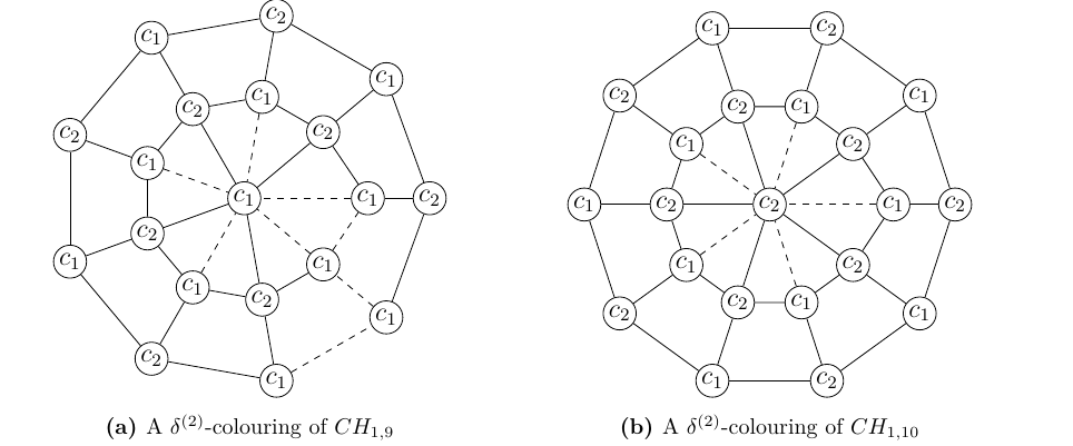
Let \(n\) be odd and \(k=3\). When \(n\) is odd \(b_3(W_{1,n})=1\). Now, the outer cycle of a \(CH_{1,n}\) can be properly coloured with \(k=3\) colours. Thus, when \(n\) is odd \(b_3(CH_{1,n})=1\)
◻
The following result discusses a \(\delta^{(k)}\)-colouring and the \(\delta^{(k)}\)-defect number of a web graph.
Definition 3. [18] A web graph, denoted by \(Wb_{1,n}\), is the graph obtained by attaching a pendant edge to each vertex of the outer cycle of the closed helm graph \(CH_{1,n}\).
It can be noted that, the vertices \(u_i\)’s and \(v_i\)’s considered in the below discussion are as per Definition 3.
Theorem 2. The \(\delta^{(k)}\)-defect number of web graph \(Wb_{1,n}\) is \[b_k(Wb_{1,n})= \begin{cases} \frac{n}{2}, & \text{if $n\geq 4$ is even and $k=2$,}\\ \lceil\frac{n}{2}\rceil+3, & \text{if $n\geq 5$ is odd and $k=2$,}\\ 1, & \text{if $n \geq 3 $ is odd and $k=3$.} \end{cases}\]
Proof. The proof of \(Wb_{1,n}\) for different parities of \(n\) and different values of \(k\) is the same as that of the proof of a \(\delta^{(k)}\)-colouring of \(CH_{1,n}\) and \(b_k(Wb_{1,n})=b_k(CH_{1,n})\) (see Theorem 1). This is because, web graph has \(n\) additional pendant vertices attached to each of the vertices of the outer cycle of \(CH_{1,n}\), which can be properly coloured with colours other than the colour assigned to its adjacent vertex. ◻
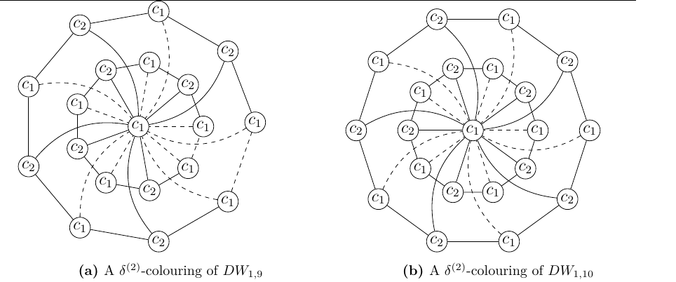
Definition 4. [17] A double wheel graph, denoted by \(DW_{1,n}\), is obtained from \(CH_{1,n}\) by adding the vertices \(u_i\); where \(1\leq i \leq n\) of \(CH_{1,n}\) to its central vertex \(v_0\), or in other words a double-wheel graph, denoted by \(DW_{1,n}\), is the graph obtained by connecting the vertices of two (disjoint) cycles each of size \(n\) to a common vertex called central vertex. That is, \(DW_{1,n}:=2C_n+K_1\).
It is to be noted that, the vertices \(u_i\)’s and \(v_i\)’s considered in the below discussion is as per Definition 4.
Theorem 3. The \(\delta^{(k)}\)-defect number of a double wheel graph \(DW_{1,n}\) is \[b_k(DW_{1,n})= \begin{cases} n, & \text{if $n\geq 4$ is even and $k=2$,}\\ 2(\lceil\frac{n}{2}\rceil+1), & \text{if $n\geq 3$ is odd and $k=2$,}\\ 1, & \text{if $n \geq 3 $ is odd and $k=3$.} \end{cases}\]
Proof. Let \(c_i\) be the available \(i\) colours with their respective colour classes \(C_i\); \(1\leq i \leq k\). Let \(v_i\) and \(u_i\); \(1\leq i \leq n\), be the vertices of the two disjoint cycles of \(DW_{1,n}\) and let \(v_0\) be the central vertex. Now, \(v_0\) is a universal vertex and hence if any colour other than the colour \(c_1\), say \(c_2\) or \(c_3\), is assigned to it, then no other \(v_i\)’s or \(u_i\)’s can be assigned the same colour to satisfy the requirements of a \(\delta^{(k)}\)-colouring of graphs. In each of the following cases different possible \(\delta^{(k)}\)-colourings are explained.
Let \(n\) be even and \(k=2\). As mentioned above two different possible \(\delta^{(2)}\)-colourings for this case are discussed. The first one is as follows. Assign the colour \(c_2\) to the vertex \(v_0\). Now, none of the remaining vertices can be assigned the colour \(c_2\) and since \(k=2\), every vertex of the two cycles are assigned the colour \(c_1\) to meet the requirements of a \(\delta^{(k)}\)-colouring of graphs. This colouring will yield \(2n\) number of monochromatic edges in \(DW_{1,n}\) (\(n\) monochromatic edges in each of the two cycles). Thus, when \(n\) is even, the \(\delta^{(2)}\)-defect number resulting from this colouring is \(2n\).
In the second \(\delta^{(2)}\)-colouring, assign the colour \(c_1\) to the vertex \(v_0\) and the vertices \(v_1, v_2,\ldots, v_n\) are properly coloured with two colours \(c_1\) and \(c_2\) alternatively. This colouring will provide a scenario where there exists no monochromatic edges in the cycle. The vertices \(u_1, u_2,\ldots, u_n\) of the outer cycle can also be coloured properly with \(k=2\) colours. Thus, the monochromatic edges in this case will arise from the vertices of both the cycles that are assigned the colour \(c_1\) incident on the central vertex \(v_0\), where \(c(v_0)=c_1\). There are each of \(\frac{n}{2}\) number of vertices that receive the colour \(c_1\) in both the cycles. Thus, there are \(n\) monochromatic edges resulting from this \(\delta^{(2)}\)-colouring. When both the above discussed \(\delta^{(2)}\)-colourings are compared, it can be observed that the second gives the minimum possible number of monochromatic edges. Thus, the \(\delta^{(2)}\)-defect number of \(DW_{1,n}\) is \(n\), when \(n\) is even (see Figure 2b for illustration).
Let \(n\) be odd and \(k=2\). The above-mentioned two \(\delta^{(2)}\)-colourings can be followed in this case as well. As explained above the first \(\delta^{(2)}\)-colouring will give rise to \(2n\) monochromatic edges. Thus, a detailed discussion on the second \(\delta^{(2)}\)-colouring is given as follows. For the second \(\delta^{(2)}\)-colouring, as explained in the second \(\delta^{(2)}\)-colouring of Case 1, the colour \(c_1\) is assigned to the vertex \(v_0\). The vertices of the two cycles are coloured with the two colours \(c_1\) and \(c_2\) alternatively. The \(\delta^{(2)}\)-defect number of odd cycles is 1 (see Proposition 2.3, [11]). Here, both the cycles will have each of one monochromatic edge. Since \(n\) is odd and \(k=2\), both the cycles will have \(\lceil\frac{n}{2}\rceil\) vertices that receive the colour \(c_1\), adjacent to the vertex \(v_0\). This results in \(\lceil\frac{n}{2}\rceil\) monochromatic edges between each of the cycles and \(v_0\). Thus, the total number of monochromatic edges obtained from the \(\delta^{(2)}\)-colouring in this case is \(2(\lceil\frac{n}{2}\rceil+1)\). Hence, when both the possible \(\delta^{(2)}\)-colourings mentioned are compared, \(b_2(DW_{1,n})=2(\lceil\frac{n}{2}\rceil+1)\), when \(n\) is odd (see Figure 2a for illustration).
Let \(n\) be odd and \(k=3\). Since there are two odd cycles of length \(n\), both can be properly coloured with three colours \(c_1, c_2\) and \(c_3\). However, as \(v_0\) is a universal vertex, it cannot be assigned any colours other than \(c_1\). Thus, between the two cycles and \(v_0\) there can be a minimum of one monochromatic edge each. Hence, there are a total of two monochromatic edges obtained from this \(\delta^{(3)}\)-colouring. Now, if the vertex \(v_0\) is given the colour other than \(c_1\), say \(c_3\), then the vertices \(v_i\)’s and \(u_i\)’s, where \(1\leq i \leq n\), of both the cycles are coloured with the colours \(c_1\) and \(c_2\). This colouring will provide one monochromatic edge in each of the odd cycles (see Proposition 2.3, [11]). Thus, this \(\delta^{(3)}\)-colouring will also result in total of two monochromatic edges in \(DW_{1,n}\). Hence, the \(\delta^{(3)}\)-defect number of \(DW_{1,n}\) is 2, when \(n\) is odd.
◻
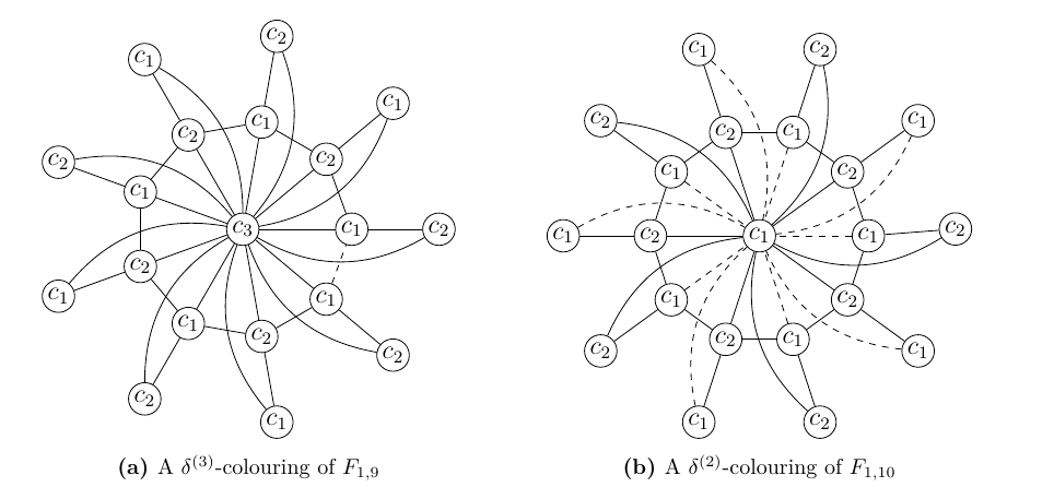
The minimum number of monochromatic edges resulting from a \(\delta^{(k)}\)-colouring of \(F_{1,n}\) is discussed in the following theorem. Since \(\chi(F_{1,n})=3\), when \(n\) is even and is 4, when \(n\) is odd, the two values that \(k\) can take are 2 and 3. A \(\delta^{(k)}\)-colouring for the different parities of \(n\) and distinct values of \(k\) is discussed in the following theorem.
Definition 5. [17] A flower graph, \(F_{1,n}\) is a graph obtained from a helm graph \(H_{1,n}\) by joining each of its pendant vertices \(u_i\)’s to its central vertex \(v_0\).
Note that, the vertices \(u_i\)’s, where \(1\leq i \leq n\), and \(v_i\)’s, where \(0\leq i \leq n\), considered in the below discussion are as per Definition 5.
Theorem 4. For a flower graph \(F_{1,n}\), the \(\delta^{(k)}\)-defect number is \[b_k(F_{1,n})= \begin{cases} n, & \text{if $n\geq 4$ is even and $k=2$,}\\ n+1, & \text{if $n\geq 3$ is odd and $k=2$,}\\ 1, & \text{if $n \geq 3 $ is odd and $k=3$.} \end{cases}\]
Proof. Let \(v_0\) be the central vertex and let \(v_1, v_2,\ldots,v_n\) be the rim vertices of the rim. Let \(u_1, u_2, \ldots, u_n\) be the pendant vertices corresponding to \(v_1, v_2,\ldots,v_n\) of the rim respectively.
A common \(\delta^{(k)}\)-colouring irrespective of the parity of \(n\) and \(k=2\) is as follows. As explained in Theorem 3, since \(v_0\) is a universal vertex, if \(c(v_0)=c_2\), then the colour \(c_2\) cannot be assigned to any of the remaining vertices. Hence, \(c_1\) is assigned to every other vertex to maintain the requirements of a \(\delta^{(k)}\)-colouring graphs and this will yield \(n\) monochromatic edges in the rim and \(n\) monochromatic edges between the cycle and the pendant vertices. Thus, when \(k=2\), the total monochromatic edges obtained from this \(\delta^{(k)}\)-colouring is \(2n\).
Now, other possible \(\delta^{(k)}\)-colourings for different parities of \(n\) and different values of \(k\) are discussed as below.
Let \(n\) be even and \(k=2\). As mentioned in the above \(\delta^{(k)}\)-colouring, the number of monochromatic edges obtained from the same is \(2n\). Now, the other possible \(\delta^{(k)}\)-colouring is investigated as follows. Assign the colour \(c_1\) to \(v_0\) and \(v_i\)’s; \(1\leq i \leq n\) are properly assigned the colours \(c_1\) and \(c_2\) alternatively. No \(u_i\)’s are adjacent to each other and hence they result in no monochromatic edges. Also, no \(u_i\)’s, adjacent to their corresponding \(v_i\)’s, are given the same colour as that of \(c(v_i)\). This results in a situation where there are no monochromatic edges between \(u_i\)’s and \(v_i\)’s. The only monochromatic edges obtained from this \(\delta^{(k)}\)-colouring is between \(v_0\) and \(v_i\)’s and \(v_0\) and \(u_i\)’s respectively. Now, there are \(\frac{n}{2}\) vertices among \(v_i\)’s and \(u_i\)’s that receive the colour \(c_1\) and this results in \(\frac{n}{2}\) monochromatic edges each. Thus, when \(n\) is even, \(b_2(F_{1,n})= n\), when both the \(\delta^{(k)}\)-colourings are compared (see Figure 3b for illustration).
Let \(n\) be odd and \(k=2\). A common \(\delta^{(k)}\)-colouring explained above result in \(2n\) monochromatic edges. A different \(\delta^{(k)}\)-colouring that results in monochromatic edges less than \(2n\) is as follows. Let \(c(v_0)=c_1\). Since \(n\) is odd, assigning the colours \(c_1\) and \(c_2\) alternatively to \(v_i\)’s, where \(1\leq i \leq n\) will results in one monochromatic edge \(v_1v_n\). Between \(v_i\)’s and \(v_0\) there are \(\lceil \frac{n}{2}\rceil\) vertices that receive the colour \(c_1\) which will cause \(\lceil \frac{n}{2}\rceil\) monochromatic edges between the same. Now, \(u_i\)’s are assigned the colours in such a way that it does not receive the colour of its corresponding \(v_i\). Assign the colour \(c_2\) to the vertex \(u_1\), \(c_1\) to the vertex \(u_2\) and so on the vertex \(u_{n-1}\) is assigned the colour \(c_2\). Since, \(c(v_n)=c_1\), \(u_n\) can be coloured with \(c_2\). Thus, there are \(\lfloor \frac{n}{2}\rfloor\) vertices among the \(n\) \(u_i\)’s that receive the colour \(c_1\). These vertices adjacent to \(v_0\) will give rise to \(\lfloor\frac{n}{2}\rfloor\) monochromatic edges. Thus, there are a minimum of \(n+1\) monochromatic edges resulting from this \(\delta^{(k)}\)-colouring. Hence, when both the \(\delta^{(k)}\)-colourings are compared, \(b_2(F_{1,n})=n+1\), when \(n\) is odd.
Let \(n\) be odd and \(k=3\). Assign the colour \(c_3\) to \(v_0\) . Since \(v_0\) is a universal vertex, none of the remaining vertices can be given the colour \(c_3\). The colour \(c_1\) and \(c_2\) are assigned to \(v_i\)’s alternatively. Since \(n\) is odd, colouring the odd cycle with two colours will result in one monochromatic edge in the cycle. Now, \(u_i\)’s are also coloured with the colours \(c_1\) and \(c_2\) as explained in Case 2. This will result in no monochromatic edges between \(u_i\)’s and \(v_i\)’s and also no monochromatic edges between \(v_0\). Thus, when \(n\) is odd, \(b_3(F_{1,n})=1\) (see Figure 3a for illustration).
◻
The below-mentioned theorem discusses a \(\delta^{(k)}\)-colouring of and the \(\delta^{(k)}\)-defect number of flower graph \(F_{1,n}\).
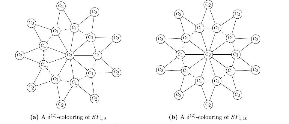
Definition 6. [17] The sunflower graph, denoted by \(SF_{1,n}\), is obtained by attaching \(n\) number of vertices \(u_i\); \(1\leq i \leq n\) corresponding to each \(v_i\), where \(1\leq i \leq n\), of \(W_{1,n}\) such that each \(u_i\) is adjacent to \(v_i\) and \(v_{i+1}\).
It is to be noted that, the vertices \(u_i\)’s and \(v_i\)’s considered in the below discussion are as per Definition 6.
Theorem 5. The \(\delta^{(k)}\)-defect number of the sunflower graph \(SF_{1,n}\) is \[b_k(SF_{1,n})= \begin{cases} n, & \text{if $n\geq 4$ is even and $k=2$,}\\ n, & \text{if $n\geq 3$ is odd and $k=2$,}\\ 1, & \text{if $n \geq 3 $ is odd and $k=3$.} \end{cases}\]
Proof. Let \(v_i\)’s, where \(1\leq i \leq n\), be the rim vertices and \(v_0\) be the central vertex of the wheel subgraph of \(SF_{1,n}\). Let \(u_i\)’s, where \(1\leq i \leq n\), be the corresponding vertices of \(v_i\). The different possible \(\delta^{(k)}\)-colourings for \(SF_{1,n}\) are discussed as follows.
Let \(n\) be even and \(k=2\). When \(k=2\), there can be two possible \(\delta^{(k)}\)-colourings for different parities of \(n\) among which one \(\delta^{(k)}\)-colouring is same irrespective of the parity of \(n\). The first \(\delta^{(k)}\)-colouring is as follows. Assign the colour \(c_1\) to the vertex \(v_1\), the colour \(c_2\) to the vertex \(v_2\), \(c_1\) to the vertex \(v_3\) and so on the colour \(c_2\) can be assigned to the vertex \(v_n\). This colouring will cause a situation where there exists no monochromatic edges in the rim. Now, \(v_0\) is assigned the colour \(c_1\) and this will result in \(\frac{n}{2}\) monochromatic edges in the wheel subgraph of \(SF_{1,n}\). Every \(u_i\) has to be assigned the colour \(c_1\) to satisfy the necessary conditions of a \(\delta^{(k)}\)-colouring of graphs which results in \(n\) monochromatic edges between \(u_i\)’s and \(v_i\)’s, where \(1\leq i \leq n\). Thus, when \(n\) is even and \(k=2\), there are a total of \(\frac{3n}{2}\) monochromatic edges obtained from the \(\delta^{(k)}\)-colouring.
Let \(n\) be odd and \(k=2\). As explained in Case 1, when \(n\) is odd and \(k=2\), there can be two possible \(\delta^{(k)}\)-colourings. The first \(\delta^{(k)}\)-colouring is as explained below. Assign the colours \(c_1\) and \(c_2\) to the rim vertices of \(W_{1,n}\) and the colour \(c_1\) is assigned to \(v_0\). This colouring will give rise to \(\lceil\frac{n}{2}\rceil\) monochromatic edges between \(v_0\) and \(v_i\), where \(1 \leq i \leq n\), and one monochromatic edge \(v_1v_n\) in the rim. Now, \(u_i\)’s, where \(1\leq i \leq n\), are assigned the colours in following manner. The colour \(c_1\) is assigned to the vertices \(u_1\) to \(u_{n-1}\) and \(u_n\) can be assigned the colour \(c_1\) or \(c_2\). In this particular case as it is adjacent to \(v_1\) and \(v_n\) which is given the colour \(c_1\), to minimise the number of monochromatic edges, assign the colour \(c_2\) is assigned to the vertex \(u_n\). This colouring will yield a situation where there are \(n-1\) monochromatic edges between \(u_i\)’s and \(v_i\)’s, where \(1\leq i \leq n\). Thus, there are a total of \(\frac{3n+1}{2}\) monochromatic edges obtained from this \(\delta^{(k)}\)-colouring when \(n\) is odd and \(k=2\).
The second \(\delta^{(k)}\)-colouring which is common for both the parities of \(n\) and \(k=2\) is discussed below. In \(SF_{1,n}\), the central vertex \(v_0\) is adjacent to all \(v_i\), where \(1 \leq i \leq n\), and all \(u_i\)’s, where \(1 \leq i \leq n\) are independent. Hence, \(v_0\) and \(u_i\)’s; \(1\leq i \leq n\), can be assigned the colour \(c_2\) and \(v_i\)’s; \(1\leq i \leq n\), can be assigned the colour \(c_1\). The monochromatic edges resulting from this \(\delta^{(k)}\)-colouring is only from the rim vertices of the wheel graph in \(SF_{1,n}\). Thus, \(b_2(SF_{1,n})\) is \(n\).
Thus, when both the \(\delta^{(k)}\)-colourings are compared, it can be seen that, the second \(\delta^{(k)}\)-colouring gives a minimum of \(n\) monochromatic edges, when \(k=2\) and irrespective of parity of \(n\). Hence, \(b_2(SF_{1,n})\) is \(n\) (see Figure 4a and Figure 4b for illustration).
Let \(n\) be odd and \(k=3\). The following explanation aims at discussing a \(\delta^{(k)}\)-colouring of \(SF_{1,n}\), when \(n\) is odd and \(k=3\). As explained above, since the vertex \(v_0\) and \(u_i\) are not adjacent to each other and since \(u_i\)’s are independent, a same colour can be given to these vertices. Since \(k=3\), assign the colour say \(c_3\) to the vertices \(v_0\) and \(u_i\). Now, \(v_i\)’s, where \(1 \leq i \leq n\), must be coloured with \(c_1\) and \(c_2\) only to meet the requirements of a \(\delta^{(k)}\)-colouring of graphs. Colour the rim of the wheel subgraph alternatively with the colours \(c_1\) and \(c_2\). This will result in a monochromatic edge \(v_1v_n\). Hence, when \(n\) is odd and \(k=3\), the \(\delta^{(k)}\)-defect number of \(SF_{1,n}\) is 1.
◻
Below-mentioned theorem investigates the \(\delta^{(k)}\)-defect number of a closed sunflower graph \(CSF_{1,n}\), for different parities of \(n\) and values of \(k\).
Definition 7. [17] A closed sunflower graph \(CSF_{1,n}\), is obtained by adding the edge \(u_iu_{i+1}\) of the sunflower graph.
Note that, in the below discussion the vertices \(u_i\)’s and \(v_i\)’s considered are as per Definition 7.
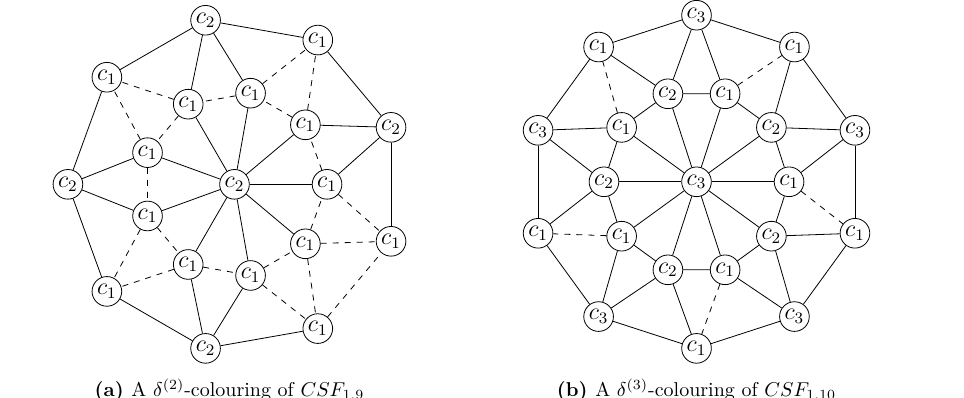
Theorem 6. The \(\delta^{(k)}\)-defect number of a closed sunflower graph \(CSF_{1,n}\) is \[b_k(CSF_{1,n})= \begin{cases} \frac{3n}{2}, & \text{if $n\geq 4$ is even and $k=2$,}\\ \frac{n}{2}, & \text{if $n\geq 4$ is even and $k=3$,}\\ \frac{5n-3}{2}, & \text{if $n\leq 7$ is odd and $k=2$,}\\ 2(n+1), & \text{if $n\geq 7$ is odd and $k=2$,}\\ \frac{n+1}{2}, & \text{if $n\geq 3$ is odd and $k=3$.} \end{cases}\]
Proof. Since \(\chi(CSF_{1,n})=4\) for any \(n\), the value of \(k\) can be 3 or 2. The different cases for different parities of \(n\) and values of \(k\) are explained as follows.
Let \(k=2\) and \(n\) be even. The first colouring for this case is colouring the even cycle properly with \(k=2\) colours and then assigning \(v_0\) and the remaining \(u_i\)’s the colour \(c_1\) to meet the requirements of a \(\delta^{(k)}\)-colouring of graphs. Thus, there are \(\frac{n}{2}\) and \(n\) monochromatic edges between \(v_0\) and \(v_i\)’s and \(v_0\) and \(u_i\)’s, where \(1\leq i \leq n\), respectively. Now, there are \(n\) monochromatic edges between \(u_i\)’s and \(v_i\)’s, where \(1\leq i \leq n\). Thus, when \(n\) is even and \(k=2\), there are \(\frac{n}{2}+n+n=\frac{5n}{2}\) monochromatic edges obtained from this \(\delta^{(k)}\)-colouring of \(CSF_{1,n}\). The second \(\delta^{(k)}\)-colouring is where \(v_0\) and the independent \(\frac{n}{2}\) vertices of \(u_i\)’s are assigned the colour \(c_2\) and the remaining \(v_i\)’s are assigned the colour \(c_1\). This colouring will give rise to situation where there are \(n\) monochromatic edges in the rim and \(n\) monochromatic edges between \(v_i\)’s and \(u_i\)’s, where \(1\leq i \leq n\). Thus, when \(n\) is even and \(k=2\), there are a total of \(2n\) monochromatic edges resulting from this \(\delta^{(k)}\)-colouring of \(CSF_{1,n}\). Thus, when the two \(\delta^{(k)}\)-colourings are compared the latter gives the minimum monochromatic edges. Hence, when \(n\) is even and \(k=2\), the \(\delta^{(k)}\)-defect number of \(CSF_{1,n}\) is \(\frac{3n}{2}\) (see Figure 5b for illustration).
Let \(k=3\) and \(n\) be even. It can be noted that, when \(n\) is even, \(\chi(W_{1,n})\) is 3 and hence the wheel subgraph of \(CSF_{1,n}\) can be properly coloured with three colours \(c_1, c_2\) and \(c_3\) as follows. Assign the colour \(c_3\) to the vertex \(v_0\) and remaining \(v_i\)’s can be properly coloured with \(c_1\) and \(c_2\) alternatively. Now, \(u_i\)’s must be coloured using only two colours \(c_1\) and \(c_3\) to maintain the requirements of a \(\delta^{(k)}\)-colouring of graphs. Thus, alternatively assign the colours \(c_1\) and \(c_3\) to \(u_i\)’s. This colouring to a situation where there will be \(\frac{n}{2}\) monochromatic edges between \(u_i\)’s and \(v_i\)’s, where \(1\leq i \leq n\). Hence, when \(n\) is odd and \(k\) is 3, the \(\delta^{(k)}\)-defect number of \(CSF_{1,n}\) is \(\frac{n}{2}\).
Let \(k=2\) and \(n\) be odd. There are two possible \(\delta^{(k)}\)-colourings that are separately discussed below.
Let \(k=2\) and \(n\) be odd. In the first colouring, as explained in Case 1, assign the colour \(c_2\) to \(v_0\) and \(\lfloor\frac{n}{2}\rfloor\) independent \(u_i\)’s. The colour \(c_1\) can be assigned to the remaining \(v_i\)’s; \(1\leq i \leq n\). Now, \(u_i\)’s when coloured with two colours will provide one monochromatic edge. There are \(\lceil\frac{n}{2}\rceil\) vertices of \(u_i\)’s that are assigned the colour \(c_1\) which will yield \(2\lceil\frac{n}{2}\rceil\) monochromatic edges between \(u_i\)’s and \(v_i\)’s, where \(1\leq i \leq n\). Also, there are \(n\) monochromatic edges in the rim of the wheel subgraph. Thus, when \(n\) is odd, \(b_2(CSF_{1,n})\) is \(2\lceil\frac{n}{2}\rceil+n+1=2(n+1)\) (see Figure 5a for illustration).
The second \(\delta^{(k)}\)-colouring is as follows. Assign the colour \(c_1\) and \(c_2\) alternatively to the rim of the wheel subgraph. Let the vertex \(v_1\) receive the colour \(c_1\), the vertex \(v_2\) the colour \(c_2\), and so on the vertex \(v_{n-1}\) is assigned the colour \(c_2\). The last vertex \(v_n\) is given the colour \(c_1\) to maintain the requirements of a \(\delta^{(k)}\)-colouring of graphs. Such a \(\delta^{(k)}\)-colouring will give rise to a monochromatic edge, say \(v_1v_n\) (see Proposition 2.4, [11]). The colour \(c_2\) cannot be assigned to the central vertex \(V_0\), and hence the colour \(c_1\) can be assigned to the central vertex to maintain the requirements of a \(\delta^{(k)}\)-colouring of graphs. This colouring will result in a situation where there exists \(\lceil\frac{n}{2}\rceil\) monochromatic edges between \(v_0\) and \(v_i\)’s, where \(1\leq i \leq n\). Now, every \(u_i\) is adjacent to the vertices \(v_i\) and \(v_{i+1}\) and hence no vertices \(u_i\) other than the vertex \(u_n\) in this case (as it is adjacent to \(v_1\) and \(v_n\) that are assigned the colour \(c_1\)) can be assigned the colour \(c_2\). Thus, there are \(n-2\) monochromatic edges in the outer cycle formed by \(u_i\)’s and \(n-1\) monochromatic edges between \(u_i\)’s and \(v_i\)’s, where \(1\leq i \leq n\). Thus, the total number of monochromatic edges in this case is \(1+\lceil\frac{n}{2}\rceil+n-1+n-2=\frac{5n-3}{2}\).
When both the colourings are compared it can be observed that, when \(k=2\) and \(n\) is odd, the \(\delta^{(k)}\)-defect number of \(CSF_{1,n}\), is \(\min\{2(n+1), \frac{5n-3}{2}\}\) which is \(\frac{5n-3}{2}\), when \(n\leq7\) and is \(2(n+1)\), when \(n\geq 7\).
Let \(k=3\) and \(n\) be odd. It is to be noted that, when \(n\) is odd, \(b_3(W_{1,n})=1\) (see Proposition 2.4, [11]). Now, two set of independent \(\lfloor\frac{n}{2}\rfloor\) vertices of \(u_i\)’s can be assigned the colour \(c_3\) and \(c_1\) to satisfy the conditions of a \(\delta^{(k)}\)-colouring of graphs. Now, the last vertex \(u_n\) which is adjacent to the vertices \(v_1\) and \(v_n\) that are assigned the colour \(c_1\) can be given the colour \(c_1\) or \(c_2\). Assigning the colour \(c_1\) will provide a scenario where there exist two monochromatic edges between the same and assigning the colour \(c_2\) will cause a situation where there is no monochromatic edge and hence \(c(u_n)=c_2\). Now, between \(u_i\)’s and \(v_i\)’s there are \(\lfloor\frac{n}{2}\rfloor\) monochromatic edges. Thus, when \(n\) is odd, \(b_3(CSF_{1,n})\) is \(1+\lfloor\frac{n}{2}\rfloor=\frac{n+1}{2}\).
◻
The following theorem determines a \(\delta^{(k)}\)-colouring and discusses the minimum number of monochromatic edges resulting from the same for different parities of \(n\) and for distinct values of \(k\) of the blossom graph, \(Bl_{1,n}\).
Definition 8. [17] A blossom graph, denoted by \(Bl_{1,n}\), is obtained by making each \(u_i\) adjacent to the central vertex of the closed sunflower graph.
Note that, the vertices \(u_i\)’s and \(v_i\)’s considered in the below discussion are as per Definition 8.
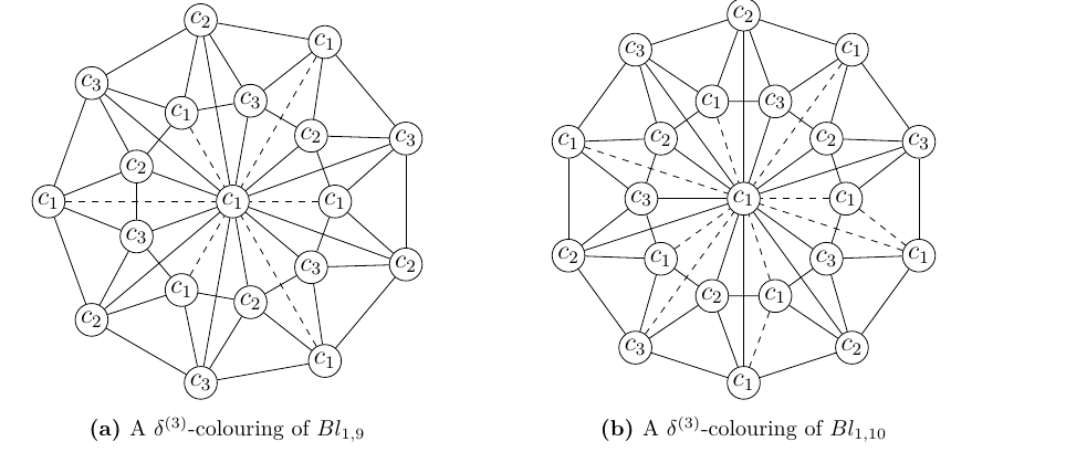
Theorem 7. The \(\delta^{(k)}\)-defect number of a blossom graph \(Bl_{1,n}\) is
\[b_4(Bl_{1,n})= \begin{cases} 2, & \text{if $n \equiv 1 \ (\mathrm{mod}\ 3) $,}\\ 1, & \text{if $n \equiv 2 \ (\mathrm{mod}\ 3) $.} \end{cases}\]
\[~~~~~~~~~~b_3(Bl_{1,n})= \begin{cases} \frac{2n}{3}, & \text{if $n \equiv 0 \ (\mathrm{mod}\ 3) $,}\\ 2\lceil\frac{n}{3}\rceil+2, & \text{if $n \equiv 1 \ (\mathrm{mod}\ 3) $,}\\ 2\lceil\frac{n}{3}\rceil+1, & \text{if $n \equiv 2 \ (\mathrm{mod}\ 3) $.} \end{cases}\] \[b_2(Bl_{1,n})= \begin{cases} \frac{7n}{2}, & \text{if $n$ is even,}\\ \frac{7n-5}{2}, & \text{if $n$ is odd.} \end{cases}\]
Proof. Let \(v_1, v_2,\ldots, v_n\) be the rim vertices of the wheel subgraph of \(Bl_{1,n}\) and \(v_0\) be its central vertex. Let \(u_1, u_2,\ldots, u_n\) be the vertices corresponding to each \(v_i\)’s, where \(1\leq i \leq n\). When \(n \equiv 1 \ (\mathrm{mod}\ 3)\) and \(n \equiv 2 \ (\mathrm{mod}\ 3)\), \(\chi(Bl_{1,n})\) is 5. Hence, for this particular case \(k\) can take the values 4, 3 and 2. When \(n \equiv 0 \ (\mathrm{mod}\ 3)\), \(\chi(Bl_{1,n})=4\), hence the value of \(k\) is 3 and 2. The various cases of a \(\delta^{(k)}\)-colourings for the different values of \(n\) and \(k\) are studied and discussed as follows.
Let \(k=4\). The minimum number of monochromatic edges obtained from a \(\delta^{(k)}\)-colouring is discussed in the following subcases.
Let \(k=4\) and \(n \equiv 1 \ (\mathrm{mod}\ 3)\). It is known that if \(n \equiv 1 \ (\mathrm{mod}\ 3)\), then \(2n \equiv 2 \ (\mathrm{mod}\ 3)\). Now, in \(Bl_{1,n}\) the central vertex \(v_0\) is a universal vertex and hence assign the colour \(c_4\) to \(v_0\). The colour \(c_4\) cannot be assigned to any of the vertices. There are three colours left to colour the remaining \(2n\) vertices. When \(k=3\), each \(2\lfloor\frac{n}{3}\rfloor\) set of disjoint independent vertices can be properly coloured with the colours \(c_1, c_2\) and \(c_3\). There are two more vertices, each of them of degree five, that are not given any colours yet. Obviously, these vertices are adjacent to the vertices assigned the colour \(c_1, c_2, c_3\) and the vertex \(v_0\) which is assigned the colour \(c_4\), by which it is also clear that they have to be assigned the colour \(c_1\) to maintain the requirements of a \(\delta^{(k)}\)-colouring of graphs. Thus, the two vertices assigned the colour \(c_1\), adjacent to two vertices assigned the same colour, will give rise to a situation where there are two monochromatic edges in the graph. Hence, when \(n \equiv 1 \ (\mathrm{mod}\ 3)\) the \(\delta^{(4)}\)-defect number of \(Bl_{1,n}\) is 2.
Let \(k=4\) and \(n \equiv 2 \ (\mathrm{mod}\ 3)\). Assign the colour \(c_4\) to the vertex \(v_0\). This colour cannot be assigned to any other vertices. The remaining \(2n\) vertices are coloured in the following manner. There are three colours left for colouring the remaining vertices. The inner and outer cycle irrespective of the parity of \(n\) are properly coloured with three colours. The monochromatic edge obtained in this case will be between \(u_i\)’s and \(v_i\)’s, where \(1\leq i \leq n\). Now, start colouring the vertices in the following pattern. Let \(c(v_1)=c_1\), \(c(v_2)=c_2\), \(c(v_3)=c_3\) and so on. This pattern is followed up to the vertex \(v_{n-2}\). The colour \(c_1\) and \(c_2\) are assigned to \(v_{n-1}\) and \(v_n\) respectively. Thus, this inner cycle is coloured properly with three colours. Now, each \(u_i\) that are adjacent to \(v_i\) and \(v_{i+1}\) are assigned a colour other than \(c(v_i)\) and \(c(v_{i+1})\). Hence, the vertex \(u_1, u_2\), \(u_3\) in this case are assigned the colour \(c_3, c_1\), \(c_2\) respectively and this colouring pattern is continued for all the remaining vertices. The vertex \(u_{n-1}\), adjacent to \(v_{n-1}\) and \(v_n\), which are assigned the colour \(c_1\) and \(c_2\), can be given the colour \(c_3\). The last vertex \(u_n\), adjacent to the vertices \(v_{n}\), \(v_{1}\), \(u_{n-1}\) and \(u_1\) which are assigned the colours \(c_2, c_1, c_3\) and \(c_3\) respectively, should be assigned the colour \(c_1\). This colouring will yield a situation where there exits a monochromatic edge \(u_nv_1\) in \(A_n\). Thus, when \(n \equiv 2 \ (\mathrm{mod}\ 3)\), the \(\delta^{(3)}\)-defect number of \(Bl_{1,n}\) is 1.
(Note that, a different \(\delta^{(k)}\)-colouring will also give \(b_k(Bl_{1,n})\geq 1\). Here, a colouring that exactly gives one monochromatic edge, which is the minimum number of monochromatic edges obtained from any improper colouring of a graph is provided)
Let \(k=3\). The different \(\delta^{(k)}\)-colourings for the different values of \(n\) when \(n \equiv i \ (\mathrm{mod}\ 3)\), where \(0\leq i \leq 2\) are discussed below.
Let \(k=3\) and \(n \equiv 0 \ (\mathrm{mod}\ 3)\). It is clear that if \(n \equiv 0 \ (\mathrm{mod}\ 3)\), then \(2n \equiv 0 \ (\mathrm{mod}\ 3)\). Here \(k=3\) and there are \(2n+1\) vertices in the graph including a universal vertex \(v_0\). If the universal vertex is given a colour other than \(c_1\), say \(c_2\) or \(c_3\), then no other vertices can be given that particular colour. Hence, to minimise the number of monochromatic edges an optimum \(\delta^{(k)}\)-colouring is as follows. Since \(2n \equiv 0 \ (\mathrm{mod}\ 3)\), the vertex set can be divided into three disjoint independent sets of order \(\frac{2n}{3}\) and assign the vertices of each set the colours \(c_1, c_2\) and \(c_3\) respectively. Now, the universal vertex \(v_0\) has to be given the colour \(c_1\) to maintain the conditions of a \(\delta^{(k)}\)-colouring of graphs. This vertex is adjacent to a total of \(\frac{2n}{3}\) vertices that are assigned the colour \(c_1\). Thus, when \(n \equiv 0 \ (\mathrm{mod}\ 3)\), the \(\delta^{(3)}\)-defect number of \(Bl_{1,n}\) is \(\frac{2n}{3}\) (see Figure 6b for illustration).
Let \(k=3\) and \(n \equiv 1 \ (\mathrm{mod}\ 3)\). It is clear that if \(n \equiv 1 \ (\mathrm{mod}\ 3)\), then \(2n \equiv 2 \ (\mathrm{mod}\ 3)\). Thus, when \(k=3\), each \(2\lfloor\frac{n}{3}\rfloor\) set of disjoint independent vertices are properly coloured with the colours \(c_1, c_2\) and \(c_3\). There are two more vertices that are of degree four which are not assigned any colours. It is obvious that these vertices are adjacent to the vertices assigned the colour \(c_1, c_2\) and \(c_3\) by which it is also clear that they have to be assigned the colour \(c_1\) to maintain the requirements of a \(\delta^{(k)}\)-colouring of graphs. Thus, the two vertices assigned the colour \(c_1\), adjacent to the two vertices having the same colour, will provide a scenario where there are two monochromatic edges in the graph. Now, \(v_0\) has to be assigned the colour \(c_1\) to meet the requirements of a \(\delta^{(k)}\)-colouring of graphs. The vertex \(v_0\) is adjacent to \(\lceil\frac{n}{2}\rceil\) vertices that are assigned the colour \(c_1\). Thus, there \(\lceil\frac{n}{2}\rceil\) monochromatic edges between \(v_0\) and \(v_i\), and \(\lceil\frac{n}{2}\rceil\) between \(v_0\) and \(u_i\). Also, there are two monochromatic edges between \(u_i\)’s and \(v_i\)’s, where \(1\leq i \leq n\). Hence, when \(n \equiv 1 \ (\mathrm{mod}\ 3)\), the \(\delta^{(3)}\)-defect number of \(Bl_{1,n}\) is \(2(\lceil\frac{n}{2}\rceil+1)\) (see Figure 6a for illustration).
Let \(k=3\) and \(n \equiv 2 \ (\mathrm{mod}\ 3)\). By Subcase 1c, it can be noted that there is only one monochromatic edge in \(Bl_{1,n}\) when \(k=4\). In this case, \(k\) is 3, and the same \(\delta^{(k)}\)-colouring as that of the one given in Subcase 1c is followed. The only difference is that since \(k=3\), the vertex \(v_0\) is assigned the colour \(c_1\) to maintain the requirements of a \(\delta^{(k)}\)-colouring of graphs. Thus, as explained in Subcase 2b, there are each of \(\lceil\frac{n}{2}\rceil\) monochromatic edges between the vertex \(v_0\) and \(v_i\) and between \(v_0\) and \(u_i\). Moreover, there is one monochromatic edge between \(u_i\)’s and \(v_i\)’s, where \(1\leq i \leq n\). Hence, when \(n \equiv 2 \ (\mathrm{mod}\ 3)\), \(b_3(Bl_{1,n})= 2\lceil\frac{n}{2}\rceil+1\).
Let \(k=2\). Following mentioned subcases discuss the different possible \(\delta^{(k)}\)-colourings for the two parities of \(n\). The \(\delta^{(k)}\)-colourings are discussed separately and compared to determine the minimum number of monochromatic edges.
Let \(k=2\) and \(n\) be even. There are two possible \(\delta^{(k)}\)-colourings for this case. In the first \(\delta^{(k)}\)-colouring, assign the colour \(c_2\) to the vertex \(v_0\). Since \(v_0\) is a universal vertex, no other vertices can be assigned the colour \(c_2\). Now, the cycles of order \(n\) formed by \(v_i\)’s and \(u_i\)’s will give rise to each of \(n\) monochromatic edges. Also, between \(u_i\)’s and \(v_i\)’s there are \(2n\) monochromatic edges. Thus, there are \(4n\) monochromatic edges obtained from this \(\delta^{(k)}\)-colouring.
In the second \(\delta^{(k)}\)-colouring, assign the vertex \(v_0\) the colour \(c_1\). Now, \(v_i\)’s are properly coloured with two colour \(c_1\) and \(c_2\) alternatively and \(u_i\)’s corresponding to each \(v_i\)’s must be coloured with colour \(c_1\) to maintain the requirements of a \(\delta^{(k)}\)-colouring of graphs. This results in \(n\) monochromatic edges between \(v_i\)’s and \(u_i\)’s, \(n\) monochromatic edges in the cycle formed by \(u_i\)’s, \(n\) monochromatic edges between \(u_i\)’s and \(v_0\), and \(\frac{n}{2}\) monochromatic edges in the inner wheel subgraph. Thus, there are a total of \(n+n+n+\frac{n}{2}=\frac{7n}{2}\) monochromatic edges. Now, when both the colourings are compared, the latter gives minimum number of monochromatic edges. Thus, when \(n\) is even, the \(\delta^{(2)}\)-defect number of \(Bl_{1,n}\) is \(\frac{7n}{2}\).
Let \(k=2\) and \(n\) be odd. There are two possible \(\delta^{(k)}\)-colourings for this case. The first one is explained as follows. As explained in Case 3a, the central vertex is given the colour \(c_2\) and every other vertex is assigned the colour \(c_1\), this \(\delta^{(k)}\)-colouring will result in \(4n\) monochromatic edges. Now, the second \(\delta^{(k)}\)-colouring is similar to the second \(\delta^{(k)}\)-colouring mentioned in Case 3a. Assign the colour \(c_1\) to the vertex \(v_0\). The inner wheel subgraph consisting of the vertices \(v_1, v_2,\ldots, v_n\) are assigned the colour \(c_1\) and \(c_2\) alternatively leading to one monochromatic edge \(v_1v_n\). Every \(u_i\) other than the vertex \(u_n\) adjacent to the monochromatic edge \(v_1v_n\), are assigned the colour \(c_1\). This colouring will result in a situation where there are \(n-1\) monochromatic edges in \(u_i\)’s, and also \(n-1\) monochromatic edges between \(u_i\)’s and \(v_0\). Moreover, there are \(n-2\) monochromatic edges between \(u_i\)’s and \(v_i\)’s, where \(1\leq i \leq n\). Thus, there are a total of \(\lceil\frac{n}{2}\rceil+n-2+n-1+n-1=\frac{7n-5}{2}\) monochromatic edges resulting from this \(\delta^{(k)}\)-colouring. Now, when both the \(\delta^{(k)}\)-colourings are compared the second \(\delta^{(k)}\)-colouring gives minimum of \(\frac{7n-5}{2}\) monochromatic edges. Hence, when \(n\) is odd, the \(\delta^{(2)}\)-defect number of \(Bl_{1,n}\) is \(\frac{7n-5}{2}\).
◻
The below-mentioned theorem examines the \(\delta^{(k)}\)-defect number of Djembe graph \(D_{1,n}\) for various values of \(k\) and different parities of \(n\). By Definition 9, it is clear that \(D_{1,n}\) has wheel graph as its subgraph.
Definition 9. [19] A djembe graph, denoted by \(D_{1,n}\), is obtained by joining the vertices \(u_i\)’s; \(1\leq i \leq n\) of a closed helm graph \(CH_{1,n}\) to its central vertex \(v_0\).
Note that, the vertices \(u_i\)’s and \(v_i\)’s considered in the below discussion are as per Definition 9.
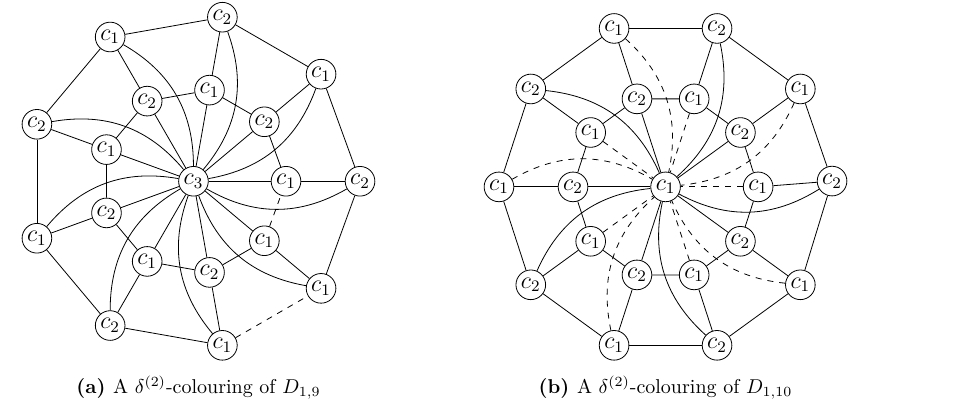
Theorem 8. For a djembe graph, the \(\delta^{(k)}\)-defect number is \[b_k(D_{1,n})= \begin{cases} n, & \text{if $n\geq 4$ is even and $k=2$,}\\ n+4, & \text{if $n\geq 3$ is odd and $k=2$,}\\ 2, & \text{if $n\geq 3$ is odd and $k=3$.} \end{cases}\]
Proof. In \(D_{1,n}\), the central vertex \(v_0\) is a universal vertex, \(v_i\)’s and \(u_i\)’s form cycles of length \(n\) and each \(u_i\) is adjacent to its corresponding \(v_i\), where \(1\leq i \leq n\). The following are the \(\delta^{(k)}\)-colourings for different parities of \(n\) and different values of \(k\).
Let \(n\) be even. Since \(\chi(D_{1,n})=3\) , the only value that \(k\) can be take is 2. There can be two possible \(\delta^{(k)}\)-colourings for this case. Since the vertex \(v_0\) is a universal vertex, \(c(v_0)=c_1\) or \(c(v_0)=c_2\). If the colour \(c_2\) is assigned to \(v_0\), then every other vertex should be given the colour \(c_1\). This colouring will cause a situation where there are each of \(n\) monochromatic edges in both cycles and \(n\) monochromatic edges between \(u_i\)’s and \(v_i\)’s, leading to a total of \(3n\) monochromatic edges. Now, if \(c(v_0)=c_1\), then since \(n\) is even, \(v_i\)’s can be properly coloured with the two colours \(c_1\) and \(c_2\). Moreover, \(u_i\)’s can be given the alternate colour of its corresponding \(v_i\). This colouring results in a scenario where there exists no monochromatic edges between \(u_i\)’s and \(v_i\)’s. Also, between \(v_0\) and \(v_i\)’s and between \(v_0\) and \(u_i\)’s there are \(\frac{n}{2}\) monochromatic edges. Thus, there are a total of \(n\) monochromatic edges resulting from this \(\delta^{(k)}\)-colouring of djembe graph. Now, when both the colouring are compared, it can be seen that, when \(n\geq 4\) is even, the \(\delta^{(2)}\)-defect number of \(D_{1,n}\) is \(n\) (see Figure 7b for illustration).
When \(n\) is odd, \(\chi(D_{1,n})=4\) and hence \(k\) is either 3 or 2. A \(\delta^{(k)}\)-colouring when \(k=2\) and \(k=3\) are separately discussed in the following cases.
Let \(n\) be odd and \(k=3\). Since \(n\) is odd, each odd cycle of order \(n\), when coloured with \(k=2\) colours will give rise to one monochromatic edge (see Proposition 2.3, [11]). Now, the colour \(c_3\) is assigned to the vertex \(v_0\). This colouring will again lead to a situation where there are no monochromatic edges between \(v_0\) and \(v_i\) and \(v_0\) and \(u_i\). Thus, when \(n\geq 3\) is odd, \(b_3(D_{1,n})\) is 2 (see Figure 7a for illustration).
Note that, in this case, any \(\delta^{(k)}\)-colouring other than the above mentioned one will also yield a minimum of two monochromatic edges as there are two odd cycles of length \(n\).
Let \(n\geq 3\) be odd and \(k=2\). As explained in Case 1, if \(c(v_0)=c_2\), then this \(\delta^{(k)}\)-colouring will lead to a situation where there are a total of \(3n\) monochromatic edges. However, if \(c(v_0)=c_1\), then there will be one monochromatic edge in each of the cycles and one monochromatic edge between \(v_i\)’s and \(u_i\)’s. The vertex \(v_0\) will provide each of \(\lceil\frac{n}{2}\rceil\) monochromatic edges between \(v_i\)’s and \(u_i\)’s. Thus, there are a total of \(2\lceil\frac{n}{2}\rceil+3\) monochromatic edges. When both the \(\delta^{(k)}\)-colourings are compared, it can be concluded that, when \(n\geq 3\), the \(\delta^{(2)}\)-defect number of \(D_{1,n}\) is \(2\lceil\frac{n}{2}\rceil+3=n+4\).
◻
In this paper, we have determined the number of bad edges for some of the wheel related graphs by discussing all the possible \(\delta^{(k)}\)-colourings and finding the optimal \(\delta^{(k)}\)-colouring that gives the minimum number of bad edges for each different values of \(k\) where \(1\leq k \leq \chi(G)-1\) from each of the graphs classes. We have permitted only one colour class to be non independent. However, permitting few more colour classes to have adjacency between the elements in it can be ground for further engrossing research.
All the authors have contributed significantly to the article. Authors declare that they don’t have any competing interests regarding the publication of this article.
They would like to thank their research colleagues Mr. Toby B Antony and Mr. Libin Chacko Samuel for their valuable inputs which significantly improved the content and the style of presentation. They also acknowledge the critical and creative comments and suggestions of the referee which improved the quality of the paper.