
All graphs discussed here are simple, finite and connected. We consider a graph \(G\) with order \(\left|V(G)\right|=p\) and size \(\left|E(G)\right|=q\). The reader can refer to Harary [1] for basic terminology in graphs. A labeling of a graph is a mapping that carries the vertices, edges or both of \(G\) to the set of non-negative or positive numbers . A mapping \(g:V(G) \rightarrow \{0,1\}\) is said to be binary labeling of \(G\) and \(g(v)\) is called label of \(v\) in \(G\) under \(g\). For any edge \(uv\), the function \(g^{*}:E(G) \rightarrow \{0,1\}\) induced by \(g\) is fixes by \(g^{*}(uv)=\left|g(u)-g(v)\right|\). Let \(v_{g}(0)\), \(v_{g}(1)\) be the count of vertices of \(G\) with label \(0\) and \(1\) respectively under \(g\). Let \(e_{g}(0)\), \(e_{g}(1)\) be the count of edges of \(G\) with label \(0\) and \(1\) respectively under \(g^{*}\). The reader can refer to Gallian [2] for getting to know a survey of graph labeling.
A pebbling move [3,4] is the removal of two pebbles from one vertex and the addition of one pebble to an adjacent vertex .
Gardner et al. [5] presented the concept of domination cover pebbling number in to the literature. The domination cover pebbling number of a graph \(G\) is \(\psi(G)\) which is the minimum number of pebbles required in such a way that any initial configuration of \(\psi(G)\) pebbles should be transformed through a number of pebbling moves such that the set of vertices with pebbles after the pebbling operation form a dominating set of \(G\).
In this paper we introduce a new concept known as binary domination cover pebbling (DCP) labeling. Also, we investigate some graphs that satisfy binary DCP labeling and give a programming approach to binary DCP labeling.
Definition 1. Let \(g:V(G) \rightarrow \{0,1\}\) be a binary labeling of \(G\) that induces a function \(g^*: E(G)\to \{0,1\}\). The function \(g\) is called a binary domination cover pebbling (DCP) labeling if \(v_g(1) + e_g(1) = \psi(G)\), where \(\psi(G)\) is the domination cover pebbling number of a graph \(G\). A graph which admits a binary domination cover pebbling (DCP) labeling is called a binary domination cover pebbling (DCP) graph.
The readers can get the information about the graphs \(W_{n}\), \(K_{1,n}\), \(F_{n}\), \(\mathbb{B}_{n}\), \(P_{n}^{2}\), \(H_{w}(n)\) and \(F_{l}(k)\) in [5-7].
In Table 1, we state the domination cover pebbling number of some families of graphs. We then determine all such graphs that admit a binary domination cover pebbling (DCP) labeling.
| Domination Cover Pebbling Number \(\psi(G)\) | Reference | |
| Path \(P_n\) | \(\left\lceil \frac{2^{n+1}-2}{7}\right\rceil\) | [8] |
| Odd Cycle \(C_2k-1\) | \(\begin{cases} \frac{2^{k+2}-9}{7} & \ \text {if} \ k=3m+5 \\ \left\lfloor \frac{2^{k+2}-1}{7}\right\rfloor & \text{ otherwise} \ k \geq 3 \ \text{and} \ \ m \geq 0 \end{cases}\) | [8] |
| Even Cycle \(C_2k\) | \(\left\lfloor \frac{3( 2^{k+1})-3}{7} \right\rfloor\) | [8] |
| Wheel graph \(W_n (n \geq 3)\) | \(n-2\) | [5] |
| Star graph \(K_1,n\) | \(n\) | [7] |
| Fan graph \(F_n, n\ge 3\) | \(n-1\) | [7] |
| Binary tree \(B_n\) | \(B_1=2\) \(B_2=11\) | [5] |
| Lollipop graph \(L_3,2\) | 3 | [9] |
| Square of path \(P_5^2\) | 3 | [6] |
| Square of path \(P_6^2\) | 5 | [6] |
| Square of path \(P_7^2\) | 6 | [6] |
| Square of path \(P_8^2\) | 9 | [6] |
| Square of path \(P_9^2\) | 10 | [6] |
| Pseudo star graph \(H_w(n)\) | \(n\) | [7] |
| Fuse graph \(F_l(k)\) | \( \begin{cases} \frac{2^{l+2}-2^{\alpha}}{7}+k-1 & \text{if} \ l-1 \equiv \alpha \neq 0 (mod 3)\\ \frac{2^{l+2}-2^{3}}{7}+k-1 & \text{if} \ l-1 \equiv 0 (mod 3) \end{cases}\) | [7] |
Lemma 1. Suppose \(G\) is a graph of order \(p\) and size \(q\), then \(v_g(1) + e_g(1) \le p + q -1\) and the bound is sharp.
Proof. By definition, it is not possible to label all the vertices and edges by 1. The upper bound is obtained. Consider the star graph \(K_{1,p-1}, p\ge 2\). If \(p=2\), label at least one vertex by 1, we get \(v_g(1) + e_g(1) = 2 = p+q-1\). If \(p\ge 3\), label only the pendant vertices by 1. Then \(v_g(1) + e_g(1) = 2p-2 = p+q-1\). ◻
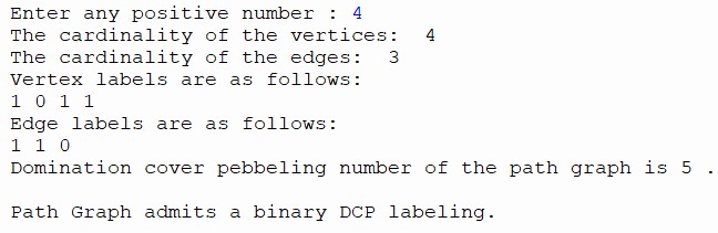
Theorem 1. The path \(P_n\) admits binary DCP labeling if \(n = 3,4\).
Proof. Suppose \(n=3\). Define \(g(a_{1})=1\) and \(g(a_{r})=0\) for \(r=2,3\). Obviously \(v_g(1) + e_g(1) =2=\psi(P_{3})\). Suppose \(n=4\). Define \(g(a_{1})=g(a_{3})=g(a_{4})=1\) and \(g(a_{2})=0\). Obviously \(v_g(1) + e_g(1) =5= \psi(P_{4})\). It is easy to see that \(P_{n}\) for \(n=3,4\) admits binary DCP labeling. ◻
def vertex1(n):
    if(i % 4 == 1):
        return 1
    else:
        return 0
def vertex2(n):
    if(i % 4 == 2):
        return 0
    else:
        return 1
def edge(i):
    if(abs(v[i-1]-v[i]) == 1):
        return 1
    else:
        return 0
n = int(input("Enter any positive number : "))
p = n
q = n-1
print("The cardinality of the vertices: ", p)
print("The cardinality of the edges: ", q)
v = [ ]
v_1 = 0
v_0 = 0
e_1 = 0
e_0 = 0
print("Vertex labels are as follows: ")
for i in range(1, p+1):
    if(n == 3):
        v.append(vertex1(i))
        print(vertex1(i), end=" ")
        if (vertex1(i)==1):
            v_1 += 1
        else:
            v_0 += 1
    elif(n == 4):
        v.append(vertex2(i))
        print(vertex2(i), end=" ")
        if (vertex2(i)==1):
            v_1 += 1
        else:
            v_0 += 1
    else:
        print("Path graph does not admit a binary DCP labeling.")
        break
if(len(v) > 1):
    print("\nEdge labels are as follows: ")
    for i in range(1,len(v)):
        print(edge(i), end=" ")
        if (edge(i)==1):
            e_1 += 1
        else:
            e_0 += 1
    print("\nDomination cover pebbling number of the path graph
is",  v_1+e_1,".")
    print("\nPath Graph admits a binary DCP labeling.")
Output
Theorem 2. The cycle \(C_n\) admits binary DCP labeling if \(n=4,6\).
Proof. Let \(C_n = a_1a_2a_3\cdots a_n\). Suppose \(n=4\). Define \(g(a_{1})=1\) and \(g(a_{r})=0\) for \(r=2,3,4\). Obviously \(v_g(1) + e_g(1) =1+2=3=\psi(C_{4})\). Suppose \(n=6\). Define \(g(a_{1})=g(a_{2})=g(a_{4})=1\) and \(g(a_{r})=0\) for \(r=3,5,6\). Obviously \(v_g(1) + e_g(1) =3+4=7=\psi(C_{6})\). Then \(C_{n}\) for \(n=4,6\) admits binary DCP labeling. ◻
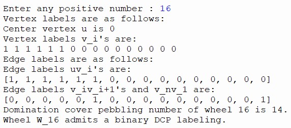
Theorem 3. The wheel graph \(W_{n}\) admits binary DCP labeling if \(n \equiv 0 \pmod{2}\) and \(n > 4\).
Proof. Let \(a\) be an apex vertex and \(a_{1},a_{2},\cdots,a_{n}\) be the rim vertices of the wheel \(W_{n}\). Suppose \(n \equiv 0 \pmod{2}\) and \(n > 4\). Define a binary labeling \(g\) that labels \(a_{1},a_{2}, \cdots ,a_{\frac{n}{2}-2}\) of rim vertices by \(1\) and remaining vertices by \(0\). Clearly, there are \(\frac{n}{2}\) edges with label \(1\). So \(v_g(1) + e_g(1) =\frac{n}{2}-2+ \frac{n}{2}=n-2=\psi(W_{n})\). Thus \(g\) is a binary DCP labeling. ◻
import math
def vertex(p) :
    if (1 <= i <= math.ceil((n-4)/2)):
        return 1
    elif (math.ceil(((n-4)/2)+1) <= i <= n):
        return 0
n = int(input("Enter any positive number : "))
v = [ ]
b = [ ]
c = [ ]
u = 0
print("Vertex labels are as follows: ")
print("Center vertex u is", u)
print("Vertex labels v_i's are: ")
for i in range(1, n+1) :
    if n > 4:
        if (n % 2 == 0):
            v.append(vertex(i))
            print(vertex(i), end= " ")
        else:
            print(f"Wheel W_{n} does not admit a binary DCP labeling.")
            break
    else:
       print(f"Wheel W_{n} does not admit a binary DCP labeling.")
       break
if len(v) >= 3:
    for i in range(1, len(v)):
        c.append(abs(u - v[i-1]))
        b.append(abs(v[i-1] - v[i]))
    c.append(abs(u - v[-1]))
    b.append(abs(v[0] - v[-1]))
    print("\nEdge labels are as follows: ")
    print("Edge labels uv_i's are: ")
    print(c, end = " ")
    print("\nEdge labels v_iv_i+1's and v_nv_1 are: ")
    print(b, end = " ")
    pebble = sum(v)+sum(b)+sum(c)
    print(f"\nDomination cover pebbling number of wheel {n} is {pebble}.")
    print("\nWheel W_{n} admits a binary DCP labeling.")
Output
Theorem 4. The star graph \(K_{1,n} \ (n \ge 2)\) admits binary DCP labeling if \(n \equiv 0 \pmod{2}\).
Proof. Suppose \(n\equiv 0\pmod{2}\). Define a binary labeling \(g\) that labels \(\frac{n}{2}\) of the pendant vertices by 1 and the remaining vertices by 0. Clearly, there are \(\frac{n}{2}\) edges with label 1. Thus, \(v_g(1)+e_g(1)=n=\psi(K_{1,n})\). This admits binary DCP labeling. ◻
Theorem 5. The fan graph \(F_{n}\) admits binary DCP labeling if \(n \equiv 0 \pmod{2}\).
Proof. Let \(a\) be the apex vertex and \(a_{1},a_{2},\cdots,a_{n}\) be the vertices of path \(P_{n}\). Suppose \(n \equiv 0 \pmod{2}\). Define a binary labeling \(g\) that labels the vertices \(a_{1},a_{2},\cdots,a_{\frac{n}{2}-1}\) by \(1\) and remaining vertices by \(0\). Clearly, there are \(\frac{n}{2}\) edges with label \(1\). \(v_g(1) + e_g(1) =\frac{n}{2}-1+ \frac{n}{2}=n-1= \psi(F_{n})\). Thus \(g\) is a binary DCP labeling. ◻
Theorem 6. The complete binary tree \(\mathbb{B}_{n}\) admits binary DCP labeling if \(n=1,2\).
Proof. Suppose \(n=1\). Let \(V(\mathbb{B}_{1})=\{v_{0},u_{1},u_{2}\}\) and \(E(\mathbb{B}_{1})=\{v_{0}u_{1},v_{0}u_{2}\}\). Define \(g(u_{1})=1\) and \(g(v_{0})=g(u_{2})=0\). Clearly, we have an edge with label \(1\). Thus \(v_g(1) + e_g(1) = 2= \psi(\mathbb{B}_1)\). Suppose \(n=2\). Let \(V(\mathbb{B}_{2})=\{v_{0}, u_{1},u_{2},w_{1},w_{2},w_{1}^{'},w_{2}^{'}\}\) and \(E(\mathbb{B}_{2})=\{v_{0}u_{1},v_{0}u_{2},u_{1}w_{1},u_{1}w_{2},u_{2}w_{1}^{'},u_{2}w_{2}^{'}\}\). Define \(g(v_{0})= g(w_{1})=g(w_{2})=g(w_{1}^{'})=g(w_{2}^{'})=1\) and \(g(u_{1})=g(u_{2})= 0\). Clearly, we have 6 edges with label \(1\). Thus \(v_g(1) + e_g(1) =11= \psi(\mathbb{B}_2)\). Thus, \(\mathbb{B}_{n}\) admits a binary DCP labeling. ◻
Theorem 7. The lollipop graph \(L_{3,2}\) admits binary DCP labeling.
Proof. Let \(L_{3,2}\) be a lollipop graph obtained from a cycle \(C_{3}, (v_{0},v_{1},v_{2})\) by attaching a path \((v_{0}u_{1})\) of length 1 to a vertex of the cycle. Define \(g(v_{1})=1\) and \(g(v_{0})=g(v_{2})=g(u_{1})=0\). Clearly, we have 2 edges with label \(1\). Thus \(v_g(1) + e_g(1) =3= \psi(L_{3,2})\). Thus, \(L_{3,2}\) admits binary DCP labeling. ◻
Theorem 8. The square \(P_{n}^{2}\) of path graph admits binary DCP labeling if \(5 \leq n \leq 9\).
Proof. Suppose \(n=5\). Define \(g(v_{1})=1\) and \(g(v_{r})= 0\), \(r\neq 1\). Clearly, we have 2 edges with label \(1\). Thus \(v_g(1) + e_g(1) =3= \psi(P_{5}^{2})\). Thus, \(P_{5}^{2}\) admits binary DCP labeling.
Suppose \(n=6\). Define \(g(v_{1})=g(v_{2})=1\) and \(g(v_{r})= 0\), \(r \neq 1,2\). Clearly, there are 3 edges with label \(1\). Thus \(v_g(1) + e_g(1) =5= \psi(P_{6}^{2})\). Thus, \(P_{6}^{2}\) admits binary DCP labeling.
Suppose \(n=7\). Define \(g(v_{1})=g(v_{7})=1\), \(g(v_{r})= 0\), \(r \neq 1,7\). Clearly, there are 4 edges with label \(1\). Thus \(v_g(1) + e_g(1) =6= \psi(P_{7}^{2})\). Thus, \(P_{7}^{2}\) admits binary DCP labeling.
Suppose \(n=8\). Define \(g(v_{1})=g(v_{2})= g(v_{3})=g(v_{8})=1\) and \(g(v_{r})= 0\), \(r \neq 1,2,3,8\). Clearly, there are 5 edges with label \(1\). Thus \(v_g(1) + e_g(1) =9= \psi(P_{8}^{2})\). Thus, \(P_{8}^{2}\) admits binary DCP labeling.
Suppose \(n=9\). Define \(g(v_{1})=g(v_{2})= g(v_{3})=g(v_{4})=g(v_{9})=1\) and \(g(v_{r})= 0\), \(r \neq 1,2,3,4,9\). Clearly, there are 5 edges with label \(1\). Thus \(v_g(1) + e_g(1) =10= \psi(P_{9}^{2})\). Thus, \(P_{9}^{2}\) admits binary DCP labeling. ◻
Theorem 9. The pseudo star graph \(H_{w}(n)\) admits binary DCP labeling if \(w=\frac{n-1}{2}\) for \(n\) is odd and \(w=\frac{n-2}{2}\) for \(n\) is even.
Proof. If \(n\) is odd, define a binary labeling \(g\) that labels the vertices \(a_{1},a_{2},\cdots, a_{\frac{n-1}{2}}\) by \(1\) and remaining vertices by \(0\). Clearly, there are \(\frac{n+1}{2}\) edges with label \(1\). So \(v_g(1) + e_g(1) =\frac{n-1}{2}+ \frac{n+1}{2}=n= \psi(H_{w}(n))\).
If \(n\) is even, define a binary labeling \(g\) that labels the vertices \(a_{1},a_{2},\cdots,a_{\frac{n}{2}}\) by \(1\) and remaining vertices by \(0\). Clearly, there are \(\frac{n}{2}\) edges with label \(1\). So \(v_g(1) + e_g(1) =\frac{n}{2}+ \frac{n}{2}=n= \psi(H_{w}(n))\). ◻
The vertices of a fuse graph \(F_{l}(k), (l \geq 2 \ \text{and} \ k \geq 2)\) are \(a_{1},a_{2} \cdots a_{n}\) with \(n=l+k\). The edges of a fuse graph are \(a_{1}a_{2},a_{2}a_{3},\cdots a_{l-1}a_{l}\) and \(a_{l}a_{l+1}, \cdots,a_{l}a_{n-1}, a_{l}a_{n}\).
Theorem 10. The fuse graph \(F_{l}(k)\) admits binary DCP labeling.
Proof. Case 1. \(l=2\) and \(k\) is odd.
We define a binary labeling \(g\)
that labels first \(\left\lceil
\frac{k}{2}\right\rceil\) vertices by \(1\) and remaining vertices by \(0\). Clearly, there are \(\left\lceil \frac{k}{2}\right\rceil\) edges
with label \(1\). So \(v_g(1) + e_g(1)
=\frac{k+1}{2}+\frac{k+1}{2}=k+1=2+k-1= \psi(F_{2}(k))\).
Case 2. \(l=3\).
Define a binary labeling \(g\) that
labels \(g(a_{1})=g(a_{2})=g(a_{3})=1\)
and \(g(a_{r})=0\), \(r \neq 1,2,3\). Clearly, there are \(k\) edges with label \(1\). So \(v_g(1)
+ e_g(1) =3+k=4+k-1= \psi(F_{3}(k))\).
Case 3. \(l=4\) and
\(2 \leq k \leq 5, k=7\).
For \(k=2\), define a binary labeling \(g\) that gives the labels \(g(a_{1})=g(a_{3})=g(a_{5})=g(a_{6})=1\) and \(g(a_{r})=0\), \(r \neq 1,3,5,6\). Clearly, there are \(2+3\) edges with label \(1\). Thus \(v_g(1) + e_g(1) =5+4=9= \psi(F_{4}(2))\).
Let \(k=3\). Define a binary labeling \(g\) that gives the labels \(g(a_{1})=g(a_{2})=g(a_{3})=g(a_{5})=g(a_{6})=g(a_{7})=1\) and \(g(a_{4})=0\). Clearly, there are \(3+1\) edges with label \(1\). Thus \(v_g(1) + e_g(1) =6+4=10= \psi(F_{4}(3))\).
Let \(k=4\). Define a binary labeling \(g\) that gives the labels \(g(a_{1})=g(a_{2})=g(a_{5})=g(a_{6})=g(a_{7})=g(a_{8})=1\) and \(g(a_{3})=g(a_{4})=0\). Clearly, there are \(4+1\) edges with label \(1\). Thus \(v_g(1) + e_g(1) =6+5=11= \psi(F_{4}(4))\).
Let \(k=5\). Define a binary labeling \(g\) that gives the labels \(g(a_{1})=g(a_{5})=g(a_{6})=g(a_{7})=g(a_{8})=g(a_{9})=1\) and \(g(a_{2})=g(a_{3})=g(a_{4})=0\). Clearly, there are \(6\) edges with label \(1\). Thus\(v_g(1) + e_g(1) =6+6=12= \psi(F_{4}(5))\).
Let \(k=7\). Define a binary labeling \(g\) that gives the labels \(g(a_{5})=g(a_{6})=g(a_{7})=g(a_{8})=g(a_{9})=g(a_{10})=g(a_{11})=1\) and \(g(a_{1})=g(a_{2})=g(a_{3})=g(a_{4})=0\). Clearly, there are \(7\) edges with label \(1\). Thus \(v_g(1) + e_g(1) =7+7=14= \psi(F_{4}(7))\). ◻
We have explored the relationship between two graph parameters namely binary labeling and domination cover pebbling. We have determined binary DCP labeling for paths, cycles, star, fan, wheel, binary tree graphs, pseudo star graph and fuse graph. It would be interesting to find other families of graphs admitting a binary DCP labeling.