
Let \(G = (V,E)=(V(G),E(G))\) be a
graph with vertex set \(V = \{v_1, v_2,
\ldots, v_n \}\) and order \(n = |V|\). The open
neighborhood of a vertex \(v\) is the set \(N(v) = \{ u | uv \in E\}\) of vertices
\(u\) that are adjacent to \(v\); the closed
neighborhood of \(v\) is
the set \(N[v] = N(v) \cup \{v \}\).
Similarly, the closed neighborhood of a set \(S\) is the set \(N[S] = \bigcup_{v \in S} N[v]\). A set
\(S \subseteq V\) is a
dominating set of \(G\) if every vertex in \(V – S\) is adjacent to at least one vertex
in \(S\), or equivalently if \(N[S] = V\). The domination
number \(\gamma(G)\) of
\(G\) equals the minimum cardinality of
a dominating set \(S\) of \(G\); we say that such a set \(S\) is a \(\gamma\)-set. For more on
domination theory, we refer the reader to [1,3].
A set \(S \subseteq V\) of vertices is
called independent if no two vertices in \(S\) are adjacent. A set \(S \subseteq V\) of vertices is called a
\(2\)-packing, or
simply a packing, if for every vertex \(v \in V\), \(|N[v] \cap S| \leq 1\), that is, no vertex
\(w \in V – S\) has two or more
neighbors in \(S\), and no vertex \(u \in S\) has a neighbor \(v \in S\). Let \(S \subset V\) be any set of vertices in a
graph \(G\), and let \(G – S\) denote the graph obtained from
\(G\) by deleting all vertices in \(S\) and deleting all edges \(uv \in E\) which are incident with a vertex
in \(S\).
An \(m \times n\) grid graph
\(G_{m,n}\) has vertex set \(V = \{(i,j) | 1 \leq i \leq m, 1 \leq j \leq n
\}\) with \((i,j)\) adjacent to
\((k,l)\) if \(i=k\) and \(|j-l|=1\) or \(j=l\) and \(|i-k|=1\). Several papers have been
published on the domination numbers of classes of grid graphs, including
[4-9].
In [4,7] the authors
prove an exact formula for the domination number of \(G_{m,n}\), for all \(m, n \ge 1\). In [10,11] the authors give methods for constructing
\(\gamma\)-sets of \(G_{m,n}\).
Let \(G = (V,E)\) be a graph. A
subset \(S \subseteq V\) of vertices is
an efficient dominating set if every vertex \(v \in V\) is adjacent to exactly one vertex
in \(S\), where a vertex \(u \in S\) is considered to be adjacent to
itself. Thus, a set \(S\) is an
efficient dominating set if for every vertex \(v \in V\), \(|N[v] \cap S| = 1\). A graph is said to be
efficient if it has an efficient dominating set.
Notice that every efficient dominating set \(S\) in a graph \(G\) is both an independent set and a \(2\)-packing. Not every graph \(G\) has an efficient dominating set. Two
simple examples are the cycles \(C_4\)
and \(C_5\), although it is easy to see
that all cycles \(C_{3k}\), for \(k \geq 1\), have efficient dominating
sets.
A dominating set \(S\) is called
total efficient if for every vertex \(v \in V\), \(|N(v) \cap S| = 1\), that is, the
open neighborhood \(N(v)\) of every vertex \(v \in V\) contains exactly one vertex in
\(S\). Not every graph \(G\) has a total efficient dominating set. A
simple example, again, is the cycle \(C_5\), although it is easy to see that all
cycles \(C_{4k}\), for \(k \geq 1\), have total efficient dominating
sets. We say that graphs having a total efficient dominating set are
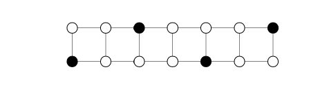
total efficient. Figure 1 illustrates an efficient
dominating set of the \(2 \times 7\)
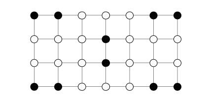
grid graph \(G_{2,7}\). Figure 2 illustrates a total efficient
dominating set of the \(4 \times 7\)
grid graph \(G_{4,7}\).
Efficient domination is of considerable importance in almost all
real-world applications of domination. Efficient dominating sets have
minimum cardinality of all dominating sets in a graph, but even more,
they dominate the vertices of a graph with no redundancy or overlap. And
thus, they provide domination at absolute minimum cost. In coding theory
efficient dominating sets are called perfect
codes, which means that they correspond to
single-error-correcting codes. This means that every vertex, or code
word, is either a member of a dominating set, or is adjacent to a unique
member of the dominating set, which represents the
single-error-corrected code word.
Although efficiency in graphs is highly desirable, in general, graphs
are usually not efficient. It is of value, therefore, to determine
optimum ways in which inefficient graphs can be changed in order to make
them efficient. One way to make an inefficient graph efficient is to
remove a minimum number \(S\) of
vertices such that the remaining graph \(G –
S\) is efficient. Thus, in this paper we will consider the
following efficiency parameter. The (vertex) efficiency
deletion number, \(\varepsilon_v^-(G)\), equals the minimum
number of vertices in a set \(S\) such
that the graph \(G – S\) is
efficient.
As discussed in Chapter 9 of [3], the current theory of efficiency in graphs is not very extensive and has focused primarily on families of graphs such as circulants, also called Cayley graphs, vertex-transitive graphs, and cube-connected cycles (cf. [3]). In 1990 Livingston and Stout [12] showed that very few grid graphs are efficient.
Theorem 1 ([12]). A grid graph \(G_{m,n}\), for \(m,n \ge 2\), has an efficient domination set if and only if either (i) \(m = n = 4\), or (ii) \(m = 2\) and \(n = 2k+1\), for any \(k \ge 1\).
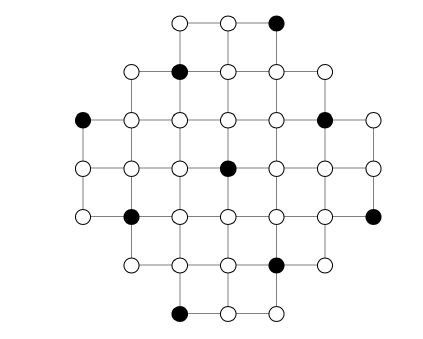
Although Theorem 1 points out that there are very few efficient grid graphs, this family of graphs is but a small subfamily of a much larger family of grid-like graphs we can call semigrid graphs, which can be defined as \(2\)-connected, plane graphs, every interior face of which is a \(4\)-cycle, as illustrated in Figure 3. It is easy to see that there are far more efficient semigrid graphs than rectangular grid graphs, as in Figure 3.
Notice in Figure 4 that the \(5 \times 5\) grid graph \(G_{5,5}\), which is not an efficient graph, is an induced subgraph of an efficient semigrid graph.
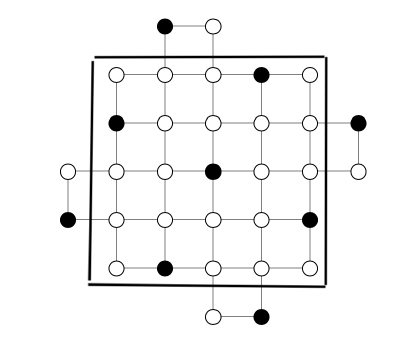
From Figure 4, the following result can easily be proved.
Theorem 2. Every \(m \times n\) grid graph \(G_{m,n}\) is an induced subgraph of an efficient semigrid graph.
Proof sketch. As illustrated in Figure 4, given an \(m \times n\) grid graph \(G_{m,n}\), select a set of vertices which creates what is called a star pattern, in which vertices are distanced from each other according to a knight’s move in chess. This pattern will efficiently dominate all vertices inside the grid, with the exception of a few vertices on the exterior which are not dominated. But these vertices can easily be efficiently dominated by augmenting the grid as indicated in Figure 4, the result of which is an efficient semigrid graph. \(\Box\)
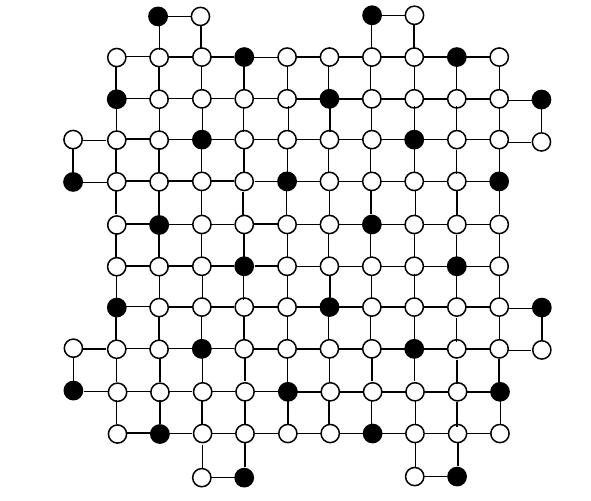
Notice in Figure 5 that the \(10 \times 10\) grid graph \(G_{10,10}\) is an induced subgraph of an
efficient semigrid graph. However, in comparison to the semigrid which
has \(G_{5,5}\) as an induced subgraph,
there are twice as many vertices exterior to the grid in Figure 5 to create an efficient
domination. Further, these exterior vertices occur either five columns
or five rows away from the previous set of exterior vertices. This
indicates that the star pattern repeats every five rows or five
columns.
As previously defined, an \(m \times n\) grid graph \(G_{m,n}\) has vertex set \(V = \{(i,j) | 1 \leq i \leq m, 1 \leq j \leq n \}\) with \((i,j)\) adjacent to \((k,l)\) if \(i=k\) and \(|j-l|=1\) or \(j=l\) and \(|i-k|=1\). We define the rectilinear distance, \(dist\), between vertices \((i,j)\) and \((k,l)\) as
\[\nonumber dist((i,j),(k,l)) = |i-k| + |j-l|.\]
We note that \(dist\) equals the
number of edges in a shortest path in \(G_{m,n}\) between \((i,j)\) and \((k,l)\).
We extend the idea of a semigrid to look at the star pattern created on
a minimally larger grid to \(G_{m,n}\)
formed by adding one row to both the top and bottom and one column to
both the left and right. Let \(G_{m+2,n+2}\) be an \((m+2) \times (n+2)\) grid graph, where
\((i,j) \in V(G_{m+2,n+2})\) if \(0 \leq i \leq m+1\) and \(0 \leq j \leq n+1\), and \(G_{m,n}\) is a subgraph of \(G_{m+2,n+2}\), such that the \((i,j)\) entry of \(G_{m,n}\) is the \((i+1,j+1)\) entry of \(G_{m+2,n+2}\). We call any vertex in \(V(G_{m+2,n+2})-V(G_{m,n})\) an exterior
vertex.
To mimic the star pattern created by an efficient dominating set on a
semigrid, as in [11], we
define a (2,1)-slant grid \(S(2,1)\) as an infinite graph with vertex
set \(V(S(2,1)) = \{ (i,j) : i \in \mathbb{Z},
j \in \mathbb{Z}\) with the property that if \((i,j) \in V(S(2,1))\) then so are \((i+2,j+1)\), \((i+1,j-2)\), \((i-2,j-1)\), and \((i-1,j+2) \}\). The edges that connect
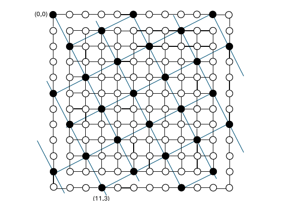
vertices \((i+2,j+1)\), \((i+1,j-2)\), \((i-2,j-1)\), and \((i-1,j+2)\) to \((i,j)\) are in the edge set \(E(S(2,1))\). Figure 6 shows a slant
grid overlayed on \(G_{m+2,n+2}\) so
that the coordinate system created by \(G_{m+2,n+2}\) is consistent with the slant
grid. To highlight \(G_{m,n}\) as a
subgraph of \(G_{m+2,n+2}\), we have
removed the edges connecting exterior vertices of \(G_{m+2,n+2}\) to vertices in \(G_{m,n}\). We note that there are 5
isomorphic graphs of \(S(2,1)\)
depending on the smallest value of \(k\), \(0 \leq k
\leq 4\) for which the vertex \((0,k)\) of \(G_{m+2,n+2}\) is a vertex of \(S(2,1)\). We denote these five slant grids
as \(S^k(2,1)\), \(0 \leq k \leq 4\). Figure 6 shows a partial
slant grid with \(k=0\), because the
slant grid intersects with vertex \((0,0)\) in the upper left corner.
Let \(V^k=V(S^k(2,1)) \cap V(G_{m+2,n+2})\). In [11] the following theorem is shown.
Theorem 3. For all \(0 \leq k \leq 4\) and all \(m,n \geq 1\), \(V^k=V(S^k(2,1)) \cap V(G_{m+2,n+2})\) is a dominating set of \(V(G_{m,n})\).
Proof. Let \((x,y) \in V(G_{m,n})\), and let \(k \in \{0,1,2,3,4 \}\). Let \((i,j) \in V^k\) so that \((i,j)\) minimizes the rectilinear distance \(dist\) to \((x,y)\). If \(dist((i,j),(x,y))= 0\), then \((x,y) = (i,j) \in V^k\). Otherwise, we wish to show that \(dist((i,j),(x,y))=1\). Assume that \(dist((i,j),(x,y)) \geq 2\). By definition of \(S^k(2,1)\), if \((i,j) \in V(S^k(2,1))\) then so are \((i+2,j+1)\), \((i+1,j-2)\), \((i-2,j-1)\), and \((i-1,j+2)\). Note that each of these 4 vertices are rectilinear distance 3 from \((i,j)\). Further, any vertex of rectilinear distance 2 to \((i,j)\) is adjacent to one of these four vertices. Hence, if \(dist((i,j),(x,y)) \geq 2\), \((x,y)\) is closer to one of \((i+2,j+1)\), \((i+1,j-2)\), \((i-2,j-1)\), and \((i-1,j+2)\) than it is to \((i,j)\), a contradiction. Hence, \(dist((i,j),(x,y)) \leq 1\) and \((x,y)\) is dominated by \((i,j) \in V^k\). \(\Box\)
Corollary 1. \(V^k\) dominates \(G_{m,n}\) so that no vertex in \(V(G_{m,n})\) is dominated more than once.
Proof. Suppose \((x,y) \in
V(G_{m,n})\) is dominated by \(v=(i,j)
\in V^k\) and \(w=(k,l) \in
V^k\). Then \(dist(v,w) =2\),
contradicting the fact that vertices in \(S^k(2,1)\) have minimum \(dist\) of 3. \(\Box\)
This corollary implies that vertices in \(V^k
\cap V(G_{m,n})\) efficiently dominate some subgraph of \(G_{m,n}\). The only vertices not dominated
are on the boundary of \(G_{m,n}\).
These vertices could be removed in order to form an efficient dominating
set for a new graph \(G'_{m,n}\),
the subgraph of \(G_{m,n}\) efficiently
dominated by \(V^k \cap V(G_{m,n})\).
Since there are five possible slant grids, \(k=0, \ldots, 4\), we seek the value of
\(k\) which minimizes the number of
vertices that we need to remove to form \(G'_{m,n}\).
In [11], the authors show
that we can move the exterior vertices in \(V^k\) to an adjacent vertex in \(G_{m,n}\) to construct a minimum dominating
set for \(G_{m,n}\) composed entirely
of vertices in \(V(G_{m,n})\). However,
moving such vertices to \(G_{m,n}\)
could create a dominating set that is not efficient because a vertex is
dominated more than once. Consider the vertex at location \((11,3)\) in Figure 6. If we move the
exterior vertex in \(V^k\), \((11,3)\), to the vertex it is dominating in
\(G_{m,n}\), \((10,3)\), we will create double-dominated
vertices at locations \((9,3)\) and
\((10,4)\). Hence, it is more efficient
just to remove vertex \((10,3)\) from
the grid in creating \(G'_{10,10}\). This is also true for
\((0,5), (5,0), (7,12) \in V^k\). In
fact, noncorner adjustments will always create two or more
double-dominated vertices when moved to \(G_{m,n}\) by the nature of the slant grid.
However, there are cases that occur at the corners of the grid graph
where we actually can remove more exterior vertices than the number of
double-dominated vertices created by moving the exterior vertex to \(G_{m,n}\).
The corner adjustment procedures in [11] will create minimum dominating sets for \(G_{m,n}\), but those dominating sets will
not be efficient since they create possibly multiple double-dominated
vertices which would need to be removed from the grid. Below, we look at
how these corner adjustments lead to grid vertex removals so that there
is an efficient dominating set of the resulting graph. We break the
cases into whether \(k\) is even or
odd.
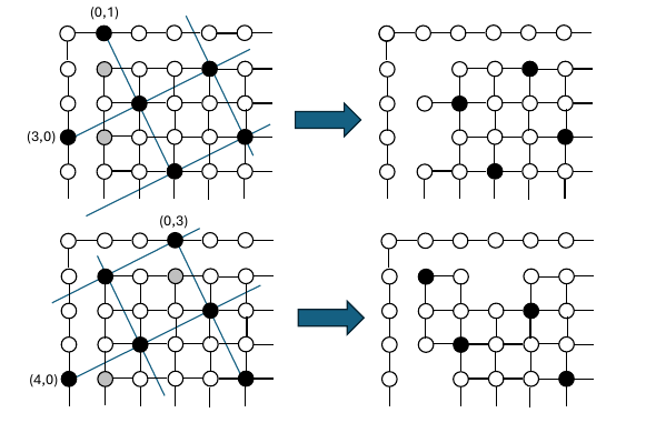
We begin with the odd cases. Figure 7 shows that when
\(k=1\), there are dominators on the
boundary at locations \((0,1)\) and
\((3,0)\). To move these dominators to
\(G_{m,n}\) in locations \((1,1)\) and \((3,1)\) creates double-dominated vertices
at \((1,2)\), \((2,1)\), and \((3,2)\). It is more efficient just to
remove vertices \((1,1)\) and \((3,1)\), shown in gray, from \(G_{m,n}\) to create efficient domination
around that corner. When \(k=3\),
Figure 7
shows that there are boundary dominators at \((0,3)\) and \((4,0)\). As before moving those vertices to
\(G_{m,n}\) creates double-dominated
vertices at \((1,2)\), \((1,4)\), \((3,1)\) and \((4,2)\). It is more efficient to just
remove the vertices \((4,1)\) and \((1,3)\), shown in gray, to create an
efficient domination of the resulting graph.
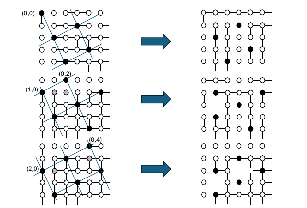
When \(k\) is even, Figure 8 shows that some efficiencies can be realized by moving boundary dominators to \(G_{m,n}\). When \(k=0\) we simply remove the boundary dominator at \((0,0)\) and \(G_{m,n}\) is still efficiently dominated around that corner. When \(k=2\), we combine the boundary dominators \((1,0)\) and \((0,2)\) to form a dominator at \((1,1)\) to create one double-dominated vertex \((2,1)\). Hence we remove two boundary dominators and only have to remove one vertex \((2,1)\) from the \(G_{m,n}\) to have efficient domination around that corner. Finally, when \(k=4\), we have two boundary dominators at \((2,0)\) and \((0,4)\). In making the adjustment from [11] to form a minimum dominating set, we move dominators at \((2,0)\) and \((1,2)\) to \((2,1)\) and \((1,3)\) respectively while removing the dominator at \((0,4)\). This removes two boundary dominators, \((2,0)\) and \((0,4)\), while creating a dominating set in \(G_{m,n}\) that double-dominates the vertices \((3,1)\) and \((2,3)\). Hence, we remove vertices \((3,1)\) and \((2,3)\) from \(G_{m,n}\) to create efficient corner domination. Note that we could just as well have removed vertices \((2,1)\) and \((1,4)\) and achieved the same net result.
In this section we use the results from the previous section to
determine an upper bound for the minimum number of vertex removals from
\(G_{m,n}\) needed to achieve an
efficient dominating set of \(G'_{m,n}\). Given \(G_{m,n}\), we overlay a slant grid \(S^k(2,1)\), for some \(k\), over \(G_{m+2,n+2}\) to form a set of vertices
that dominate the vertices in \(G_{m,n}\), but not all of them are
contained in \(G_{m,n}\). Any vertex in
\(v \in V(G_{m,n})\) that is dominated
by an exterior vertex in \(V(G_{m+2,n+2}) –
V(G_{m,n})\) will be a potential vertex to be removed from \(G_{m.n}\). In fact, if \(v\) is not located around a corner of \(G_{m,n}\), then it is most efficient to
remove \(v\) from \(V(G_{m,n})\) (along with its incident
edges). Around the corners of \(G_{m,n}\), when \(k\) is odd or \(k=4\), we will also just remove the vertex
\(v\). However, when \(k=0\) or \(k=2\), we actually remove more vertices
from the boundary for every double-dominated vertex created. Hence, we
would like to maximize the number of times we have the opportunity to
create the scenarios at a corner where \(k=0\) or \(k=2\).
Before that discussion, if we could count the number of dominators that
are on the exterior and subtract off the number of dominators not on the
exterior, this would give us an upper bound on the number of vertices
needed to be removed from \(G_{m,n}\)
in order for the dominators in \(V^k \cap
V(G_{m,n})\) to form an efficient dominating set. This upper
bound can be lowered by four vertices if each corner adjustment results
in cases where \(k=0\) or \(k=2\). In [11], we show that
\[\left\lfloor \frac{(m+2)(n+2)}{5} \right\rfloor \leq |V^k| \leq \left\lfloor \frac{(m+2)(n+2)}{5} \right\rfloor +1.\]
By extension of this idea, it follows that
\[\left\lfloor \frac{(m)(n)}{5} \right\rfloor \leq |V^k \cap V(G_{m,n})| \leq \left\lfloor \frac{(m)(n)}{5} \right\rfloor +1.\]
Combining these two ideas above, we have the following.
Lemma 1. If \(\varepsilon_v^-(G_{m,n})\) is the minimum number of vertices that need to be removed from \(V(G_{m,n})\) in order to create an efficient graph, then
\[\varepsilon_v^-(G_{m,n}) \leq \Big( \left\lfloor \frac{(m+2)(n+2)}{5} \right\rfloor +1 – \left\lfloor \frac{(m)(n)}{5} \right\rfloor \Big).\]
This bound can be improved further by maximizing the number of
adjustments at the corners that lead to more removals from the boundary
of \(G_{m+2,n+2}\) than would need to
be removed from \(G_{m,n}\), i.e. cases
where the corners have an abundance of \(k=0\) or \(k=2\) cases. In what follows, we show, for
each \(4 \leq m \leq 8\) and \(n\geq m\), the configuration of the slant
grid (choice of \(k\)) that allows for
the minimum number of vertices to be removed from the grid graph to
create an efficient subgraph in this way.
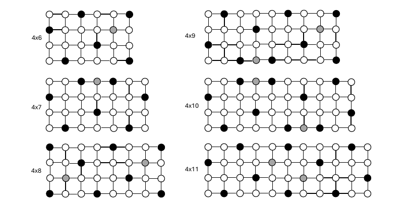
When \(m=4\), in Figure 9, we show that \(k=0\) allows for the same case to show up
in the lower left portion of the grid as well. For the grid graph \(G_{4,4}\) this scenario shows up in all
four corners. By inspecting all five possibilities (\(k=0,1,2,3,4\)), we can see that this case
minimizes the number of grid vertices needed to be removed in order to
achieve efficient domination in the resulting graph. When \(n=4\), we note that we remove zero vertices
to achieve efficient domination, as was noted in [12]. As \(n\) progresses from 4 to 8, we see that the
corners on the right-hand-side of the figures have different
configurations. Upon removing the vertices as dictated by the specific
type of corner adjustment, we create efficient augmented grids.
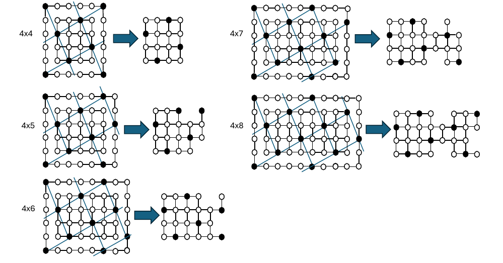
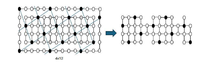
Note that in the \(4 \times 9\) case (not shown), that the corner removals present in the \(4 \times 4\) case reappear, allowing for only the removal of two vertices (those present in the interior of the \(4 \times 7\) and \(4 \times 8\) cases). Likewise, the \(4 \times 10\) case will have the same corner removal pattern as the \(4 \times 5\) case, and so on. However, the \(4 \times 10\) case will have two more vertices removed compared to the \(4 \times 5\) case, namely vertices at locations \((1, 5)\) and \((4,5)\). So, the same corner removal pattern will appear from these five starting positions for every increase in \(n\) by 5. For each increase in \(n\) by 5, we will need to remove two extra interior vertices of the grid graph as compared to \(4 \times (n-5)\). To illustrate this more concretely, compare the removal pattern for \(G_{4,12}\) in Figure 10 to the removal pattern of \(G_{4,7}\) in Figure 9 to see that the corner adjustments are the same but two extra vertices at \((1,10)\) and \((4,10)\) must be removed in forming \(G'_{4,12}\) because of the cyclical pattern in slant grids. We have indicated the vertices \((1,5), (4,5), (1,10)\), and \((4,10)\) in gray.
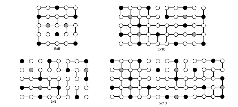
When \(m=5\), the corner configuration in the upper left corner that works best for \(n=5, 6, 7, 8\) is when \(k=2\) as shown in Figure 11. By inspection, every other value of \(k\) either removes the same number of vertices or more.
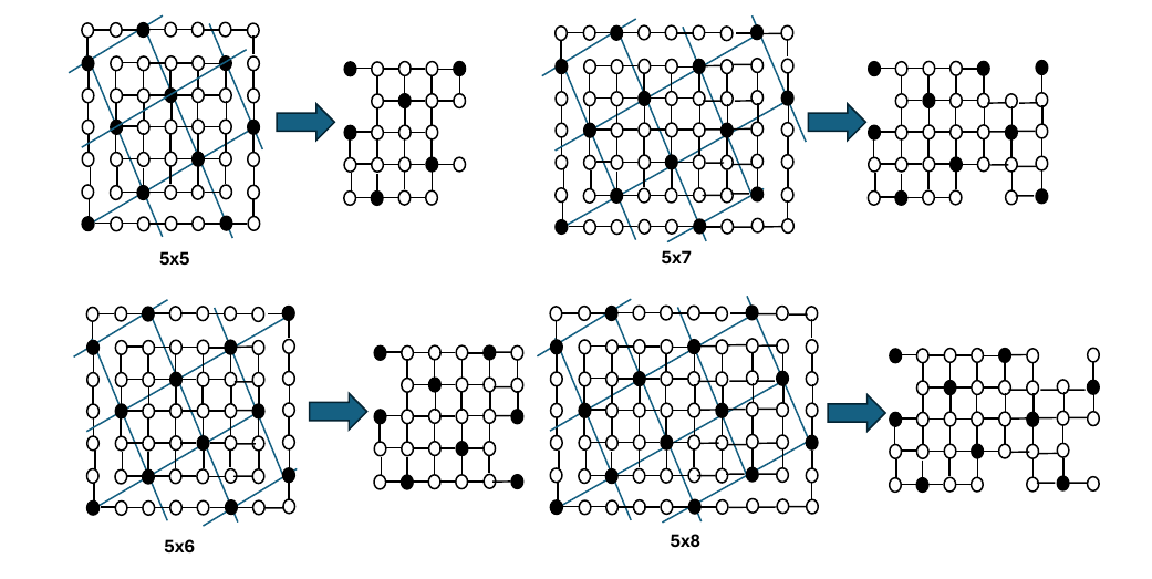
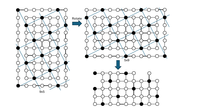
It is interesting to note that we do not show the ideal case for \(G_{5,9}\). This is because a dimension of nine is five units more than a dimension of four. If we look at \(G_{9,5}\) the corner configurations that works best are the same as the case for \(G_{4,5}\). To get the best corner configuration for \(G_{5,9}\) we would flip the grid along the \(m=n\) axis. We show this in Figure 12.
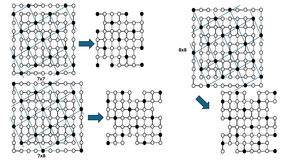
When \(m=6\), we only show the best corner configurations for \(G_{6,6}\), \(G_{6,7}\), and \(G_{6,8}\) as configurations of \(G_{6,9}\) and \(G_{6,10}\) are the same as \(G_{4,6}\) and \(G_{5,6}\), respectively. Further, corner configurations for \(G_{6,11}\), \(G_{6,12}\), and \(G_{6,13}\) are the same as \(G_{6,6}\), \(G_{6,7}\), and \(G_{6,8}\) respectively. The patterns then repeat for an increase in \(m\) or \(n\) by five. The minimum number of vertex removals from these corner configurations are shown in Figure 13.
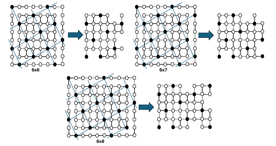
Finally, as before, we only need to show the optimal corner configurations for \(G_{7,7,}\), \(G_{7,8}\) and \(G_{8,8}\), since other configurations for these values of \(m\) can be found as extensions of cases where \(m=4, 5, 6\). These corner configurations inspire vertex removals as shown in Figure 14.
From the base cases shown in Figures 9 through 14 we can show how vertex removals grow as \(m\) and \(n\) increase by five. Table 1 shows the minimum number of vertices which need to be removed from \(G_{m,n}\) using this slant grid method. This will serve as an upper bound for \(\varepsilon_v^-(G_{m,n})\) in these cases.
| Grid Graph | No. Vertices Removed | Grid Graph | No. Vertices Removed |
| \(G_4,4\) | 0 | \(G_5,8\) | 4 |
| \(G_4,5\) | 2 | \(G_6,6\) | 4 |
| \(G_4,6\) | 2 | \(G_6,7\) | 4 |
| \(G_4,7\) | 3 | \(G_6,8\) | 4 |
| \(G_4,8\) | 3 | \(G_7,7\) | 4 |
| \(G_5,5\) | 3 | \(G_7,8\) | 4 |
| \(G_5,6\) | 2 | \(G_8,8\) | 5 |
| \(G_5,7\) | 3 |
For every increase of \(m\) or \(n\) by five we will have to remove two vertices from the grid graph since slant grid dominators appear on the boundary of \(G_{m+2,n+2}\) every five columns or rows. Hence, we can summarize the upper bounds on vertex removals for \(G_{m,n}\) with the following result.
Theorem 4. Given \(m,n \geq 4\), Table 2 gives upper bounds on the minimum number of vertices to be removed from \(G_{m,n}\) so that the resulting graph has an efficient dominating set. This table assumes that \(i\) and \(j\) are non-negative integers.
| Grid Graph | UB for\(\varepsilon_v^-(G_m,n)\) |
| \(G_5i+4,5j+4\) | \(0 + 2i + 2j\) |
| \(G_5i+4,5j+5\) | \(2 + 2i + 2j\) |
| \(G_5i+4,5j+6\) | \(2 + 2i + 2j\) |
| \(G_5i+4,5j+7\) | \(3 + 2i + 2j\) |
| \(G_5i+4,5j+8\) | \(3 + 2i + 2j\) |
| \(G_5i+5,5j+5\) | \(3 + 2i + 2j\) |
| \(G_5i+5,5j+6\) | \(2 + 2i + 2j\) |
| \(G_5i+5,5j+7\) | \(3 + 2i + 2j\) |
| \(G_5i+5,5j+8\) | \(4 + 2i + 2j\) |
| \(G_5i+6,5j+6\) | \(4 + 2i + 2j\) |
| \(G_5i+6,5j+7\) | \(4 + 2i + 2j\) |
| \(G_5i+6,5j+8\) | \(4 + 2i + 2j\) |
| \(G_5i+7,5j+7\) | \(4 + 2i + 2j\) |
| \(G_5i+7,5j+8\) | \(4 + 2i + 2j\) |
| \(G_5i+8,5j+8\) | \(5 + 2i + 2j\) |
While Theorem 4 provides general upper bounds for cases when \(m,n \geq 4\), we can improve those bounds in specific cases. As the authors in [11] point out, for some values of \(m\), minimum dominating sets are found by repeatedly flipping the dominating structure of a \(\gamma\)-set. For example, Figure 9 shows the minimum dominating set for a \(4 \times 4\) grid. This \(\gamma\)-set is also efficient. In [11] the authors show that the optimal \(\gamma\)-set for a \(4 \times 7\) grid is the \(\gamma\)-set for a \(G_{4,4}\) reflected over column four of the grid, producing the \(\gamma\)-set seen in Figure 15. Note that this \(\gamma\)-set can be made efficient by removing the vertex \((1,4)\) shown in gray in the figure.
In fact, this idea of repeatedly flipping/reflecting the \(\gamma\)-set for \(G_{4,4}\) creates an optimal \(\gamma\)-set for \(G_{4,4+3k}\), \(k\geq 0\). These \(\gamma\)-sets have a double-dominated vertex that needs to be removed for each reflection in order to make the \(\gamma\)-set produce an efficient dominating set. This is shown for \(G_{4,7}\) and \(G_{4,10}\) in Figure 15 and \(G_{4,13}\) in Figure 16.
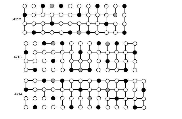
There is a simple pattern that emerges for creating efficient domination from \(G_{4,k}\) when \(k\) is not of the form \(4+3i\). Note that for \(G_{4,3k}\) we see the same pattern of reflected dominators as with \(G_{4, 3k-2}\) with the last two columns the same as the last two columns of \(G_{4,6}\). For \(G_{4,3k+2}\), \(k \geq 1\), while \(G_{4,8}\) has a slightly different pattern, \(G_{4,11}\)’s domination pattern is to take the pattern for \(G_{4,6}\) and reflect the pattern over the sixth column and then flip this pattern (the last five columns) again vertically. For \(G_{4,14}\) we take the dominating pattern for \(G_{4,6}\) and attach a reflected and flipped pattern from \(G_{4,6}\) to account for the last five columns (as we did for \(G_{4,11}\)). We can continue to do this for each of of the grids \(G_{4,3k+2}\). Note that the gray dots dominate the vertices that would need to be removed for efficient domination in these grids. Note that the removed vertices grow at a rate of one removal for every pattern “flip” and thus is a rate of one removal for every three columns, which is lower than the rate of \(\frac{2}{5}\) as in Theorem 2. Table 3 summarizes these upper bound improvements.
| Grid Graph | \(k\) | UB for \(\varepsilon_v^-(G_m,n)\) |
| \(G_4,4+(3k-1)\) | \(k \geq 1\) | \(k\) |
| \(G_4,4+(3k)\) | \(k \geq 1\) | \(k\) |
| \(G_4, 4+(3k+1)\) | \(k \geq 1\) | \(k+1\) |
When \(m=5\), there are several cases where we can improve upon the bounds given in Theorem 4, namely when \(n=5k\) or \(n=5k+3\). While \(G_{5,5}\) is a special case, considerthe dominating set for \(G_{5,8}\) in Figure 17. This dominating set creates the need to only remove three vertices from the grid instead of four given by Theorem 4. Notice that in creating a dominating set from \(G_{5,10}\), we take the dominating set for \(G_{5,8}\) and attach two extra columns with a flipped dominating pattern of the first two columns of the dominating set of \(G_{5,8}\). To create the dominating set for \(G_{5,13}\), we take the dominating set for \(G_{5,8}\) and flip columns three through seven over column eight to create the dominating pattern for columns nine through thirteen. In each of these we create dominating sets which become efficient when removing the gray vertices and require fewer vertex removals than Theorem 4 requires.
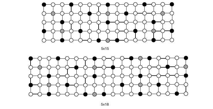
In Figure 18, the creation of a minimum dominating set for \(G_{5,15}\) involves taking the dominating pattern for \(G_{5,8}\) and reflecting the first seven columns over column eight. Further, the dominating set for \(G_{5,18}\) takes the dominating set for \(G_{5,13}\) and reflects columns eight through twelve over column thirteen to create the dominating pattern for \(G_{5,18}\). This reflecting pattern continues for all grids of the form \(G_{5,5k}\) and \(G_{5,5k+3}\).
Note that the number of vertices that need to be removed grows at the same rate that is described in Theorem 4, which is two removals for every five columns. However, \(G_{5,5}\) and \(G_{5,8}\) has a dominating set which requires fewer removals than described by Theorem 4, namely two and three respectively rather than three and four. Table 4 describes the number of vertex removals needed per value of \(k\) when \(m=5\).
| Grid Graph | \(k\) | UB for\(\varepsilon_v^-(G_m,n)\) |
| \(G_5,5k\) | \(k \geq 1\) | \(2k\) |
| \(G_{5,5k+3}\) | \(k \geq 1\) | \(2k+1\) |
When \(m=6\), Figure 19 shows that we can do better than the bounds described in Theorem 4 for the cases where \(n=6\) and \(n=7\). For each of these two, we can create efficient dominating sets for that only require removing three vertices instead of four. Then, using a similar slant grid approach, we must remove two vertices for every five column we add from that point. So, in creating an efficient domination for \(G_{6,11}\) and \(G_{6,12}\), Figure 19 shows what those dominating sets would look like. This pattern will continue for grids of the form \(G_{6,6+5k}\) and \(G_{6,7+5k}\).
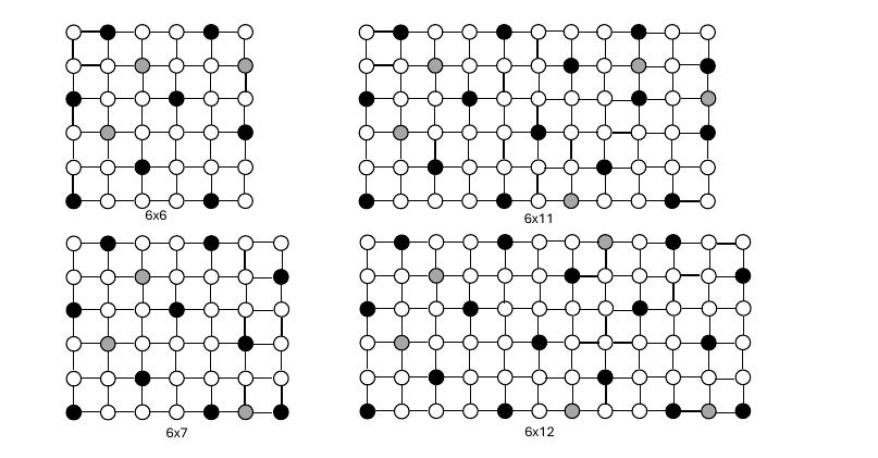
Table 5 summarizes these improvements to the upper bounds for \(\varepsilon_v^-(G_{m,n})\) for certain cases where \(m=6\).
| Grid Graph | \(k\) | UB for \(\varepsilon_v^-(G_{m,n})\) |
|---|---|---|
| \(G_{6,6+5k}\) | \(k \geq 1\) | \(3+2k\) |
| \(G_{6,7+ 5k}\) | \(k \geq 1\) | \(3+2k\) |
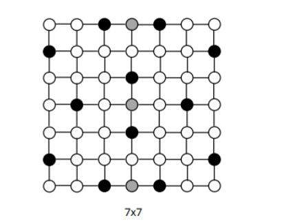
Finally, when \(m=7\), there is one case where we can achieve a better upper bound on \(\varepsilon_v^-(G_{7,k})\) than described in Theorem 4. It is the case when \(k=7\). Figure 20 shows that we can flip the optimal domination pattern for \(G_{4,7}\) over row four and create a \(\gamma\)-set for \(G_{7,7}\) which requires only three vertices to be removed to achieve efficient domination.
To check the optimality of these results, we created the following
integer programming model and ran it through a solver (glpk) to find the
minimum number of vertices which would need to be removed to achieve
efficient domination for \(G_{m,m}\),
for all values of \(4 \leq m,n \leq
16\). It verified that the upper bound either achieved by
Theorem 4 or the tables in this section were indeed
optimal. However, we do not currently have an approach to prove this
result.
in formulating the integer program, we set up three types of decision
variables. We let \(x(i,j)\) be a
binary variable indicating whether or not the vertex at \((i,j)\) will be selected as a dominator for
\(G'_{m,n}\). We let \(y(i,j)\) be a binary variable indicating
whether or not the vertex at \((i,j)\)
will be removed because it is not being dominated. Finally, we let \(z(i,j)\) be an integer variable indicating
how many times the vertex at \((i,j)\)
will be dominated. If \(z(i,j) > 1\)
in the optimal solution, then we reduce the solution to one, since it
could not be removed more than once. For each of these variables, \(1 \leq i \leq m\) and \(1 \leq i \leq n\).
Integer Programming Model for \(\varepsilon_v^-(G_{m,n})\)
min \(\sum_{i=1}^m
\sum_{j=1}^n (y(i,j) + z(i,j))\)
s.t.
Constraints for the Corners
\(x(1,1) + x(2,1) + x(1,2) = 1 – y(1,1)
+z(1,1),\)
\(x(1,n) + x(1,n-1) + x(2,n) = 1 -y(1,n) +
z(1,n),\)
\(x(m,1) + x(m-1,1)+ x(m,2) = 1 – y(m,1) +
z(m,1),\)
\(x(m,n) + x(m-1,n) + x(m,n-1) = 1 – y(m,n) +
z(m,n),\)
Constraints for the Non-Corner Sides of the Grids
\(x(i,1) + x(i-1, 1) +x(i+1, 1) + x(i,2) = 1 –
y(i,1) + z(i,1), \hspace{0.1in} 2 \leq i \leq m-1,\)
\(x(i,n) + x(i-1,n) + x(i+1,n) + x(i,n-1) = 1
– y(i,n) + z(i,n), \hspace{0.1in} 2 \leq i \leq m-1,\)
\(x(1,j) + x(1,j-1) + x(1,j+1) + x(2,j) = 1 –
y(1,j) + z(1,j), \hspace{0.1in} 2 \leq j \leq n-1,\)
\(x(m,j) + x(m,j-1) + x(m,j+1) + x(m-1,j) = 1
-y(m,j) + z(m,j), \hspace{0.1in} 2 \leq j \leq n-1,\)
Constraints for the Interior of the Grid
\(x(i,j)+ x(i-1,j) + x(i+1,j) + x(i,j-1) +
x(i,j+1) = 1- y(i,j) + z(i,j), \hspace{0.1in} 2 \leq i \leq m-1, 2 \leq
j \leq n-1,\)
\(x(i,j), y(i,j) \in \{0,1\}\), \(1 \leq i \leq m\), \(1 \leq j \leq n,\)
\(z(i,j)\) integer, \(1 \leq i \leq m\), \(1 \leq j \leq n\).
In this paper, we have established upper bounds on the vertex efficiency deletion number for grid graphs. These bounds were found using a construction approach in [11] designed to create \(\gamma\)-sets for grids. These approaches were modified to indicate which vertices in a grid graph need to be removed in order to create efficient domination from vertices that appear in a slant grid pattern within the grid. Although there are multiple slant grid overlays, we indicate the one for each value of \(m \geq 4\) leading to the minimum number of vertices which need to be removed from \(G_{m,n}\), for each \(n \geq 4\), that leaves an efficient resulting graph.
For certain values of \(m\) and \(n\), the bounds given in Theorem 4 could be improved. Using an integer programming model as a guide, we found improvements to the upper bounds listed in Theorem 4. Although we believe the bounds listed in this paper are the exact value for \(\varepsilon_v^-(G_{m,n})\) for \(m,n \geq 4\), it is still an open question to find proofs for this.
Further, we have focused on removing vertices from the grid to produce efficient domination in the resulting graph. However, we could ask what is the smallest efficient semigrid, one having no leaves, that contains a given grid \(G_{m,n}\) as an induced subgraph. In other words, what is the minimum addition to the grid that results in an efficient semigrid. In addition, our approach to create the upper bounds in Theorem 4 removed vertices on the exterior boundary of \(G_{m,n}\). However, we found improvements for certain cases that allowed interior vertices to be removed. We might ask if there are ways to achieve efficient domination for grids where only interior vertices are removed. As a quick example, \(G_{3,5}\) has an efficient domination when the interior vertex at location \((2,3)\) is removed.