$e$-injective coloring: $2$-distance and injective coloring conjectures

1. Introduction

Graph coloring has many applications in various fields of life, such as timetabling, scheduling daily life activities, scheduling computer processes, registering allocations to different institutions and libraries, manufacturing tools, printed circuit testing, routing and wavelength, bag rationalization for a food manufacturer, satellite range scheduling, and frequency assignment. These are many applications that are out there right now and many more come in the follow.

A proper $k$-coloring (hereafter $k$-coloring) of a graph $G$ is a function $f:V(G)\to \{1,2,3,\dots ,k\}$ such that for all edge $xy\in E$, $f(x)\ne f(y)$. The chromatic number of $G$, denoted by $\chi (G)$, is the minimum integer $k$ such that $G$ has a $k$-coloring. There are many research works on the graph coloring parameters that is not possible to name all of them here. For instance see [4,17].

In $1969$, Kramer and Kramer introduced the notion of $2$–distance coloring of a graph $G$ or the usual proper coloring of $G^2$ [9], we can some of its applications in [10]. A $2$–distance $k$-coloring of a graph $G$ is a function $f:V\to \{1,2,3,\dots ,k\}$, such that no pair of vertices at distance at most $2$, receive the same color, in the other words, the colors of the vertices of all $P_3$ paths in the graph are distinct. The $2$-distance chromatic number of $G$, denoted by ${\chi }_2(G)=\chi (G^2)$, is the minimum positive integer $k$ such that $G$ has a $2$-distance $k$-coloring. The $2$-distance coloring of $G$, is a proper coloring [3,2,5].

For a graph $G$, the subset $S$ of $V(G)$ is said to be a dominating set if any vertex $x\in V\setminus S$ is adjacent to a vertex $y$ in $S$. A dominating set of $G$ with minimum cardinality is called the domination number of $G$ and is denoted by $\gamma (G)$. A subset $D$ of $V(G)$ is said to be $2$-distance dominating set if any vertex $d\in V\setminus D$, is in at most $2$-distance of to a vertex in $D$. A $2$-distance dominating set of $G$ with minimum cardinality is called the $2$-distance domination number of $G$ and is denoted by ${\gamma }_2(G)$.

The injective coloring was first introduced in $2002$ by Hahn et al. [6] and it was also further studied in [1,8,11,12,15,16,18]. An injective $k$-coloring of a graph $G$ is a function $f:V\to \{1,2,3,\dots ,k\}$ such that no vertex $v$ is adjacent to two vertices $u$ and $w$ with $f(u)=f(w)$, in the other words, for any path $P_3=xyz$, we have $f(x)\ne f(z)$. The injective chromatic number of $G$, denoted by ${\chi }_i(G)$, is the minimum positive integer $k$ such that $G$ has an injective $k$-coloring. The injective chromatic number of the hypercube has important applications in the theory of error-correcting codes. As it is well known, the injective coloring of $G$, is not necessarily proper coloring. Injective coloring of a graph $G$ is related to the usual coloring of the square $G^2$. The inequality ${\chi }_i(G)\le {\chi }_2(G)$ obviously holds.

There are several results related to injective coloring that review the usual coloring results in graph theory from a new point of view, in particular on the injective chromatic number of planar graphs. As well, many conjectures on planar graphs have been posed and studied by authors so far. In this regard, we bring up some of them as follows.

From the relation between the injective coloring of a graph $G$ and the usual coloring of the square $G^2$, Wegner [19] posed the following conjecture.

Lužar and Škrekovski in [11] showed that:

Adapted from Theorem 1.2, they proposed the following Wegner type conjecture for the injective chromatic number of planar graphs.

By the relation between injective chromatic number and $2$-distance chromatic number of a graph; showing the truth of Conjecture 1.1 (parts (2), (3)), will deduce the truth of Conjecture 1.3 (parts (ii), (iii)).

Now we introduce a new concept of vertex coloring (near to injective coloring) as an $e$-injective coloring of a graph. The motivation of the alleging is to study, how it behaves against of the injective graph coloring, usual graph coloring, $2$-distance graph coloring, packing set, dominating set and $2$-distance dominating set of graphs. As well, in particular we investigate the posed conjectures from the point of view of $e$-injective colorings. Also since the notion of $e$-injective coloring is near to injective coloring, one can predict, it has applications in various fields of life in real world and would also be useful in coding theory as so did injective coloring.

This concept is introduced in next definition.

Hereafter, we say that, two vertices $u,v$ have a common edge neighbor if there exist an edge $e$ in which, $u$ is adjacent to one end vertex of $e$ and $v$ is adjacent to another end vertex of $e$.

The $e$-injective coloring of $G$, is not necessarily proper coloring. This concept can be expressed as new discourse.

From the point of view of $e$-injective coloring, the type of Conjectures 1.1 and 1.3 can be declared as a problem, which can be argued in next section.

In the sequence, we assume that all graphs in this paper are finite, simple, and undirected. We use [4,20] as a reference for terminology and notation which are not explicitly defined here. Throughout the paper, we consider $G=(V,E)$ be a finite simple graph with vertex set $V=V(G)$ and edge set $E=E(G)$. The open neighborhood of a vertex $v\in V$ is the set $N(v)=\{u|uv\in E\}$, and its closed neighborhood is the set $N[v]=N(v)\cup \{v\}$. The cardinality of $|N(v)|$ is called the degree of $v$, denoted by $\mathrm{deg}(v)$. The minimum degree of $G$ is denoted by $\delta (G)$ and the maximum degree by $\mathrm{\Delta }(G)$. A vertex $v$ of degree $1$ is called a pendant vertex or a leaf, and its neighbor is called a support vertex. A vertex of degree $n-1$ is called a full or universal vertex while a vertex of degree $0$ is called an isolated vertex.

For any two vertices $u$ and $v$ of $G$, we denote by $d_G(u,v)$ the distance between $u$ and $v$, that is the length of a shortest path joining $u$ and $v$. The path, cycle and complete graph with $n$ vertices are denoted by $P_n$, $C_n$ and $K_n$ respectively. The complete bipartite graph with $n$ and $m$ vertices in their partite sets is denoted by $K_{n,m}$, while the wheel graph with $n+1$ vertices is denoted by $W_n$. A star graph with $n+1$ vertices, denoted by $S_n$, consists of $n$ leaves and one support vertex. A double star graph is a graph consisting of the union of two star graphs $S_m$ and $S_n$, with one edge joining their support vertices; the double star graph with $m+n+2$ vertices is denoted by $S_{m,n}$.

The join of two graphs $G$ and $H$, denoted by $G\vee H$, is the graph obtained from the disjoint union of $G$ and $H$ with vertex set $V(G\vee H)=V(G)\cup V(H)$ and edge set $E(G\vee H)=E(G)\cup E(H)\cup \{xy|x\in V(G),y\in V(H)\}$. A fan graph is a simple graph consisting of joining ${\overline{K}}_m$ and $P_n$; the fan graph with $m+n$ vertices is denoted by $F_{m,n}$. For two sets of vertices $X$ and $Y$, the set $[X,Y]$ denotes the set of edges $e=uv$ such that $u\in X$ and $v\in Y$.

The square graph $G^2$ is a graph with the same vertex set as $G$ and with its edge set given by $E(G^2)=\{uv|dist(u,v)\le 2\}$. The chromatic number $\chi (G^2)$ of $G^2$ (or $2$-distance chromatic number ${\chi }_2(G)$ of $G$) has been studied extensively in planar graph [7,14].

A subset $B\subseteq V(G)$ is a packing set in $G$ if for every pair of distinct vertices $u,v\in B$, $N_G[u]\bigcap N_G[v]=\mathrm{\varnothing }$. The packing number $\rho (G)$ is the maximum cardinality of a packing set in $G$.
A subset $B\subseteq V(G)$ is an open packing set in $G$ if for every pair of distinct vertices $u,v\in B$, $N_G(u)\bigcap N_G(v)=\mathrm{\varnothing }$. The open packing number ${\rho }^{\circ }(G)$ is the maximum cardinality among all open packing sets in $G$.

Let $G$ and $H$ be simple graphs. For three standard products of graphs $G$ and $H$, the vertex set of the product is $V(G)\times V(H)$ and their edge set is defined as follows:

• In the Cartesian product $G\mathrm{<img\; draggable="false"\; role="img"\; class="emoji"\; alt="◻"\; src="https://s.w.org/images/core/emoji/15.1.0/svg/25fb.svg">}H$, two vertices are adjacent if they are adjacent in one coordinate and equal in the other.

• In the direct product $G\times H$, two vertices are adjacent if they are adjacent in both coordinates.

• The edge set of the strong product $G⊠H$, is the union of $E(G\mathrm{<img\; draggable="false"\; role="img"\; class="emoji"\; alt="◻"\; src="https://s.w.org/images/core/emoji/15.1.0/svg/25fb.svg">}H)$ and $E(G\times H)$.

In the end of this section, we explore the purpose of the paper as follows. In Section 2, we study ${\chi }_{ei}(G)$ versus to the $\chi (G)$, ${\chi }_2(G)$ and ${\chi }_i(G)$, as well, we review the conjectures raised so far in the literature of injective and $2$-distance colorings, from the new approach, $e$-injective coloring, and by disproving the Problem 1.6, we show that the Conjectures 1.1 and 1.3 maybe wrong under the conditions. For disjoint graphs $G,H$, with non-empty edge sets, ${\chi }_{ei}(G\cup H)=max\{{\chi }_{ei}(G),{\chi }_{ei}(H)\}$ and ${\chi }_{ei}(G\vee H)=|V(G)|+|V(H)|$. The $e$-injective chromatic number of $G$ versus of the maximum degree and packing number of $G$ is investigated, and denote $max\{{\chi }_{ei}(G),{\chi }_{ei}(H)\}\le {\chi }_{ei}(G\mathrm{<img\; draggable="false"\; role="img"\; class="emoji"\; alt="◻"\; src="https://s.w.org/images/core/emoji/15.1.0/svg/25fb.svg">}H)\le {\chi }_2(G){\chi }_2(H)$ in Section 3. In Section 4, we prove that, for any tree $T$ ($T\ne S_n$), ${\chi }_{ei}(T)=\chi (T)$, and we obtain the exact value of $e$-injective chromatic number of some special graphs and finally, we end the paper with discussion on research problems.

2. On the two conjectures

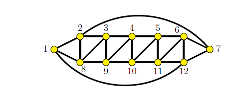
We maybe cannot compare ${\chi }_{ei}(G)$ with $\chi (G)$, $\mathrm{\Delta }(G)$, ${\chi }_i(G)$ or ${\chi }_2(G)$ in general. For instance, ${\chi }_{ei}(K_3)=1$ while $\chi (K_3)=3={\chi }_i(K_3)={\chi }_2(G)$; or ${\chi }_{ei}(K_{1,n})=1$ while $\chi (K_{1,n})=2,{\chi }_i(K_{1,n})=n$ and ${\chi }_2(K_{1,n})=n+1$. But in the Figure 1, ${\chi }_{ei}(G)=12$, ${\chi }_i(G)\le 7$, ${\chi }_2(G)\le 7$, $\chi (G)=3$.

Also let $H=K_m⊚K_n$ be a graph obtain from two complete graphs $K_m$ and $K_n$ ($m\ge n\ge 4$) with joining one vertex of $K_m$ to one vertex of $K_n$. Then $\chi (H)=m={\chi }_i(H)$, ${\chi }_2(H)=m+1$ and ${\chi }_{ei}(H)=m+n-1$ (see Proposition 4.4). On the other hand, for Complete graph $K_n$ ($n\ge 4$), odd cycle $C_{3k}$ for odd $k\ge 1$, we have ${\chi }_{ei}(K_n)=n=\chi (K_n)={\chi }_i(K_n)={\chi }_2(K_n)$, and ${\chi }_{ei}(C_{3k})=3=\chi (C_{3k})={\chi }_i(C_{3k})={\chi }_2(C_{3k})$.

In the same way, we have $\mathrm{\Delta }(K_3)=2$, $\mathrm{\Delta }(H)=m$, and for graph $G$ in Figure 1, $\mathrm{\Delta }(G)=4$, while ${\chi }_{ei}(K_3)=1$, ${\chi }_{ei}(H)=m+n-1$, and ${\chi }_{ei}(G)=12$. On the other hand, for graph $K_n⊚K_1$ ($n\ge 4$) and even cycle $C_{2k}$, we have ${\chi }_{ei}(K_n⊚K_1)=n=\mathrm{\Delta }(K_n⊚K_1)$, and ${\chi }_{ei}(C_{2k})=2=\mathrm{\Delta }(C_{2k})$ (see Proposition 4.3).

However we have the following.

Also, we may have.

Now we discuss on the Problem 1.6. Below figures denote that the Problem 1.6 is not necessarily true. On the other hand the type of Conjectures 1.1, 1.3 are not true for $e$-injective coloring. But if we use the Propositions 2.2, 2.3, then maybe characterize graphs $G$ in which, satisfy on the Conjectures 1.1, 1.3 and also characterize graphs $G$ in which, the Conjectures 1.1, 1.3 are not true for them.

Disprove of Problem 1.6
Let $G$ be a planar graph with maximum degree $\mathrm{\Delta }$. Then we present counterexample that denote the Problem 1.6 is not true.

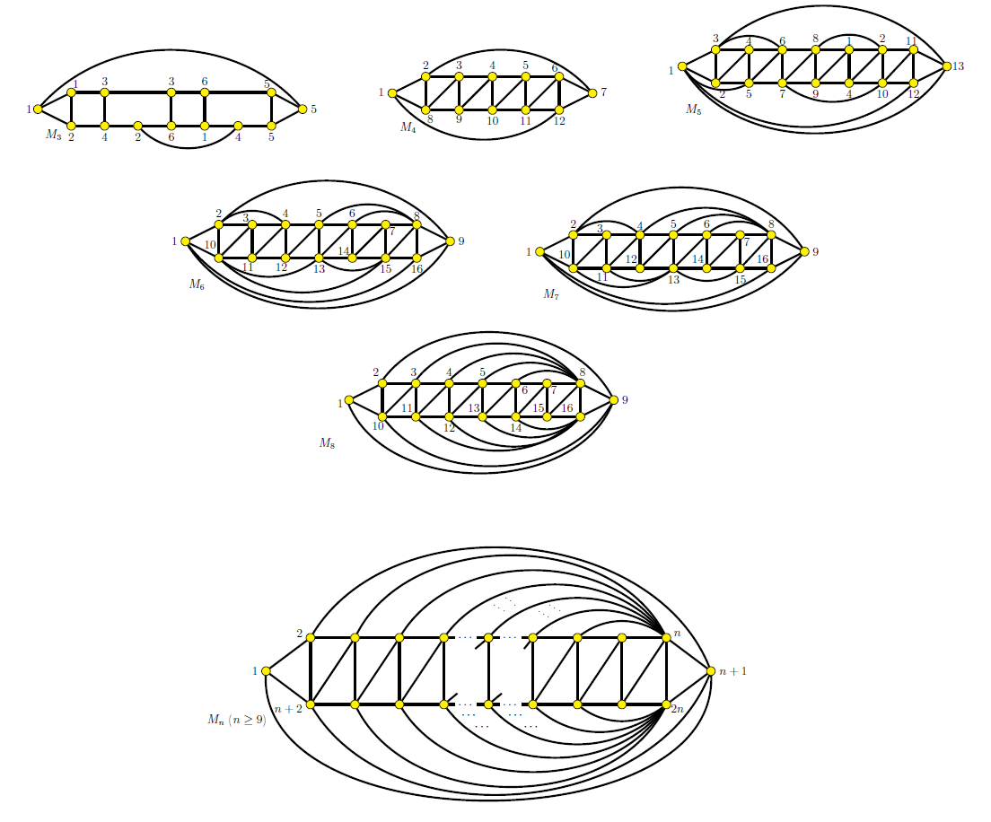
As we observe the Figure 2, for ($3\le \mathrm{\Delta }\le 8$) we have.

The graph $M_3$ denotes a planar graph in which $\mathrm{\Delta }(M_3)=3$ and ${\chi }_{ei}(M_3)=6>5$.

The graph $M_4$ denotes a planar graph in which $\mathrm{\Delta }(M_4)=4$ and ${\chi }_{ei}(M_4)=12>\mathrm{\Delta }(M_4)+5$.

The graph $M_5$ denotes a planar graph in which $\mathrm{\Delta }(M_5)=5$ and ${\chi }_{ei}(M_5)=13>\mathrm{\Delta }(M_5)+5$.

The graph $M_6$ denotes a planar graph in which $\mathrm{\Delta }(M_6)=6$ and ${\chi }_{ei}(M_6)=16>\mathrm{\Delta }(M_6)+5$.

The graph $M_7$ denotes a planar graph in which $\mathrm{\Delta }(M_7)=7$ and ${\chi }_{ei}(M_7)=16>\mathrm{\Delta }(M_7)+5$.

For $\mathrm{\Delta }(G)=8$, consider the graph $M_8$ of order $16$, which is seen $\mathrm{\Delta }(G)=8$ and ${\chi }_{ei}(M_n)=16>\lfloor \frac{24}{2}\rfloor +1=13=\lfloor \frac{3\mathrm{\Delta }}{2}\rfloor +1$.

For $\mathrm{\Delta }(G)\ge 9$ consider, the graph $M_n$ ($n\ge 9$) of order $2n$, Figure 2, which is seen $\mathrm{\Delta }(G)=n$ and ${\chi }_{ei}(M_n)=2n>\lfloor \frac{3n}{2}\rfloor +1=\lfloor \frac{3\mathrm{\Delta }}{2}\rfloor +1$.

With this regard, the Problem 1.6 is disproved. In the other words the type of Conjecture 1.3 for $e$-injective coloring is rejected. However, from the Propositions 2.2 and 2.3, we can have.

3. $e$-injective chromatic number on operation of graphs

In this section we prove some results on $e$-injective coloring using some operations.

For graphs $G$ and $H$, let $G\cup H$ be the disjoint union of $G$ and $H$. Then it is easy to see that ${\chi }_{ei}(G\cup H)=max\{{\chi }_{ei}(G),{\chi }_{ei}(H)\}$.

For the join of two graphs, we have the following.

Let $G$ be a graph and $B$ be a maximum packing set of $G$. If $v\in V(G)\setminus B$, then there is a vertex $u\in B$ such that $N(v)\cap N(u)\ne \mathrm{\varnothing }$. This shows that, $d(v,u)\le 2$. Thus $B$ is a $2$-distance dominating set. Therefore we have.

We now give an upper bound on ${\chi }_{ei}(G)$ that may be slightly important.

Also we want to drive bounds for the $e$-injective coloring of Cartesian product of two graphs $G$, $H$ in terms of $2$-distance coloring of the of $G$ and $H$. For this we explore a result from [13] and a lemma.

Now we have the following.

Theorem 3.6. For any graphs $G$ and $H$ with no isolated vertices, with the property that, any two end vertices of each path $P_4$ in $G$ and $H$ are adjacent or have a common neighbor, we have $$Max\{{\chi }_{ei}(G),{\chi }_{ei}(H)\}\le {\chi }_{ei}(G\mathrm{<img\; draggable="false"\; role="img"\; class="emoji"\; alt="◻"\; src="https://s.w.org/images/core/emoji/15.1.0/svg/25fb.svg">}H)\le {\chi }_2(G){\chi }_2(H).$$ The bounds are sharp.

4. $e$-injective chromatic number of special graphs

In this section we investigate the $e$-injective coloring of some special graphs, such as trees, path, cycle, complete graphs, wheel graphs, star, complete bipartite graphs, $k$-regular bipartite graphs, multipartite graphs and fan graphs.

As an immediate from Theorem 4.1 we have.