Research on the construction of financial market volatility prediction model in digital economy environment based on machine learning algorithm

1. Introduction

With the continuous development of the financial market, predicting the volatility of the financial market has become one of the core issues in the study of finance. In finance, volatility usually refers to the degree of market price or index changes, which is an important reflection of risk in the market [5,18,1,8]. The prediction of financial market volatility is also of great significance in the formulation of investment and trading strategies. Therefore, the research and construction of financial market volatility prediction model has always been one of the hot spots and difficulties in finance research [28,13,6,3].

The volatility of the financial market has many complex reasons, such as political, economic and natural disasters and other factors, which may directly or indirectly lead to the turbulence and volatility of the financial market. Therefore, the prediction of financial market volatility can not only help investors and traders to formulate effective risk management strategies, but also help the government to guide and regulate the healthy development of financial markets [22,23,10,4]. In addition, the prediction of market volatility is also important in the regulation of financial markets and the formulation of regulatory policies. Common financial market volatility prediction models include time series-based models, models based on variance decomposition and covariance decomposition, and models based on autoregressive conditional heteroskedasticity models [17,25,11,9]. All of these models model and predict volatility from different perspectives, and the predictive results of these models are affected by historical data, thus the volatility prediction of the future market tends to have high accuracy [16,14].

Yang et al. [29] introduced volatility as an important indicator of market risk and emphasized the importance of studying and forecasting volatility of high-frequency data. Modeling the jump volatility of high-frequency data was proposed for short-term volatility prediction of high-frequency data. Wang et al. [24] constructed a hybrid model combining GARCH model and LSTM neural network to improve the prediction of financial market volatility. An empirical analysis based on the CSI300 dataset indicates that the hybrid model improves the forecasting performance of VaR compared with the traditional GARCH model. It shows that hybrid models combining mathematical models and economic mechanisms have benefits such as enhanced portfolio risk management. Behera et al. [2] extend the discussion of using machine learning techniques to predict financial market volatility to the real estate market context. Aspects such as methods and case studies for predicting real estate market volatility are discussed. Practical applications of machine learning in predicting real estate market volatility are demonstrated for stakeholders. Xu et al. [27] explored the approach of combining deep learning with classical econometric models to address the challenge of predicting the risk of financial market volatility and proposed a framework combining LSTM and GARCH. The validation based on the historical data of NASDAQ 100 index shows that the fusion model outperforms other models in terms of prediction accuracy. Pan et al. [19] introduced a domain-adaptive financial market volatility prediction method based on the construction of a single-domain financial product volatility prediction model, FinWaveNet, and extended the method. The effectiveness of this method in volatility prediction in the financial domain was verified based on ablative and comparative experiments. Lin et al. [15] proposed a volatility forecasting methodology based on SP-M-Attention, which has several advantages such as being “suitable for long time series analysis tasks”. Based on a financial market dataset in order to validate the effectiveness of this approach, the results emphasize that the predictive performance of the model is higher than that of all benchmark models, which is beneficial for financial risk management and optimization of investment strategies.

In order to examine the data characteristics of financial market volatility more accurately, this paper analyzes the volatility data from the dimensions of price relationship, volatility data outliers, and long-term dependence, which lays the foundation for accurately constructing the financial market volatility prediction model. The importance of the features is compared by Boruta algorithm to evaluate the predictive ability of the model. SHAP analysis is used to explain the degree of contribution of features to the prediction results. Combine the two in order to improve the accuracy and interpretability of financial data feature selection. Input layer, Dropout layer, LSTM layer, connection layer, and full connection layer are designed respectively to construct AMP-LSTM model to predict the financial market volatility, and Adam optimization method is chosen to control the gradient dropout, and then relevant indexes are combined to analyze the prediction ability of the constructed model in terms of arithmetic examples.

2. Analysis of financial data sets

Owing to the uncertainty and complexity of financial markets, volatility data often have outliers and long-term dependence, and volatility is an indicator of the nature of price fluctuations. Therefore, it is necessary to comprehensively analyze volatility data from three aspects: price relationships, volatility data outliers and long-term dependence. This can help to construct more accurate and effective volatility forecasting models.

2.0.1. Price relationship analysis

. Analyzing the price relationship can reflect the predictive significance of volatility, because there is a certain relationship between volatility and price, and when volatility rises, price usually rises as well, and vice versa. Therefore, analyzing from the perspective of price relationship can better understand the trend of volatility rise and fall and its forecasting significance, and provide reference for the construction of volatility forecasting model.

According to the analysis of the data of the SSE 50ETF fund, when the volatility of the 50ETF fund rises, the price of the 50ETF flat option will also rise. Therefore, investors can choose to buy call options or sell put options to get higher benefits. On the contrary, when the volatility of the 50ETF fund decreases, the price of the 50ETF option also decreases, and the investor can choose to purchase put options or sell call options for higher benefits. Therefore, 50ETF fund volatility is an important indicator that 50ETF option investors must pay attention to.

Due to the influence of many factors such as politics, economy and investor psychology, financial time series have a lot of noise and uncertainty. This complexity makes financial time series analysis very challenging. In this context, STL time series decomposition is an applicable analytical method for financial time series, especially considering the internal complexity of financial data. Compared with other analysis methods, the most attractive feature of STL can be that it focuses on the internal characteristics of financial data by decomposing them into trend, period and residual components [20]. Among them, the trend component is used to describe the overall trend of the time series, the period component is used to describe the cyclical changes in it, and the residuals contain the parts of the time series that are not explained by the trend and the period, which include factors such as noise and outliers.

2.0.2. Analysis of volatility data outliers

.

By analyzing volatility data outliers, noise and outliers in the data can be removed to improve the accuracy and robustness of the model for better volatility forecasting.

The volatility of the SSE 50 ETF fund has been in a constant state of fluctuation, and this trend is not monotonically rising or falling, but is unstable and nonlinear, which makes it necessary for the model to be able to capture the nonlinear features in order to better predict the future trend. Noise and outliers can affect the accuracy and robustness of the model, so data need to be detected and processed for outliers.

For the noise and outliers present in the residual component part, these outliers can adversely affect the modeling, so robust outlier detection methods are needed to accurately identify and remove outliers. Median Absolute Deviation (MAD) is applicable to univariate sample data and is a robust outlier detection method.

MAD is defined as the median of the absolute deviations from the median of the sample and Eq. (1) is given below: $$\begin{array}{}\text{(1)}& MAD=median(|X_i-median(X)|),\end{array}$$ where $median(X)$ is the median of the factor values. Compared to the standard deviation, the MAD method is more resilient to outliers in the sample data and can reduce the impact of outliers on the sample data. Therefore, in this subsection, the MAD method is used for outlier detection. The MAD method is based on the median calculation, which is more robust compared to replacing the outliers with the mean, because the median has less impact on the extreme values in the dataset, and finally the resulting outliers will be replaced by the median [12].

2.0.3. Analysis of long-term dependence of volatility data

. Volatility data, such as that of the SSE 50 ETF, is often characterized by long-term dependence, which means that past events may have an impact on future changes over a longer period of time. Analyzing volatility data from the perspective of long-term dependence can better capture its characteristics and construct suitable time series models to more accurately predict future volatility movements. Therefore, it is very important to analyze volatility data from the perspective of long-term dependence in financial time series analysis.

R/S analysis is an analysis method based on the Hurst index, which was initially proposed by H.E. Hurst, a British scholar in the early 20th century, in his study of the water volume of the Nile River, and is called the coup time scale analysis method. The core idea of the method is to use the change of time scale to transform the regularity of small-scale time scale into large-scale range of research, or to apply the regularity of large-scale time scale to small-scale research in order to study the change rule of the statistical characteristics of the object, so as to reveal the long-term dependence effect and memory cycle of various natural phenomena, including the application of analysis in the field of finance. This subsection verifies the long-term dependence of the volatility of the SSE 50 ETF fund through the Hurst index.

The steps of R/S analysis method are as follows:

(1) Given a volatility series of $\{v_1,v_2,\dots ,v_N\}$ and $N$ as the length of the data.

(2) Calculate the average of the first $u$, $v$, ${\overline{v}}_u=\frac{1}{u}\sum _{j=1}^u{v}_j,u=1,2\dots N$.

(3) Determine the cumulative deviation: $X_{\tau },u=\sum _{j=1}^r(v_j-{\overline{v}}_u),\tau =1,2,\dots ,N$.

(4) Calculate $R_u=max(X_{\tau ,u})-min(X_{\tau ,u}),\tau =1,2,\dots ,N$.

(5) Calculate the standard deviation of $S_u=((u-1{)}^{-1}\sum _{j=1}^r((v_j-{\overline{v}}_u{)}^2){)}^{\frac{1}{2}}$.

(6) Set $u\le n\le N$ and apply $(log\left(\frac{R_u}{S_u}\right),logu)(u=n-k+1,n-k+2,\dots ,n)$.

$k$ is the width of the slider, do linear regression, and get the Hurst value by the least squares method.

According to the calculation results, the Hurst value of the volatility of the SSE 50 ETF fund is 0.9382. When the Hurst index is greater than 0.5, it indicates that the time series is characterized by long-term dependence, and the closer the Hurst index is to 1, the stronger the dependence is. Therefore, it is proved that the time series has a strong long-term dependence, and this paper is constructing a forecasting model, in order to predict the future volatility trend more accurately, it is necessary to consider the time series model to capture its long-term dependence.

3. Financial data characterization and forecasting

3.1. Boruta SHAP model construction

Feature selection is a key step in financial time series forecasting for selecting features with predictive power and eliminating redundant features. The Boruta-SHAP method is used as the feature selection module, which combines the Boruta feature selection algorithm with the SHAP analysis method to improve the accuracy and interpretability of feature selection.

The Boruta algorithm evaluates the predictive power of each feature by comparing its importance to that of a randomly generated “shadow” feature [7], whereas the SHAP analysis method provides an interpretation of the features to help understand the extent to which the features contribute to the prediction results [21]. The steps of the Boruta-SHAP algorithm are as follows. .

(1) Data initialization, a copy of each feature in the original dataset is created, these new features mimic the original features and eliminate their correlation with the corresponding variables, and then these added features are randomly disrupted to eliminate their correlation with the corresponding variables. This operation ensures that there is no real correlation between the newly added features and the target variables and avoids introducing bias in the feature selection process: the matrix before and after initialization is as follows: $$\begin{array}{}\text{(2)}& \left(\begin{array}{cccc}{x}_{11}& x_{12}& \cdots & x_{1n}\\ x_{21}& x_{22}& \cdots & x_{2n}\\ ⋮& ⋮& \ddots & ⋮\\ x_{n1}& x_{n2}& \cdots & x_{nn}\end{array}\right),\end{array}$$ $$\begin{array}{}\text{(3)}& \left(\begin{array}{cccc}{x}_{11}& x_{12}& \cdots & x_{1n}\\ x_{21}& x_{22}& \cdots & x_{2n}\\ ⋮& ⋮& \ddots & ⋮\\ x_{m1}& x_{m2}& \cdots & x_{mn}\\ shado{w}_{11}& shado{w}_{12}& \cdots & shado{w}_{1n}\\ shado{w}_{21}& shado{w}_{22}& \cdots & shado{w}_{2n}\\ ⋮& ⋮& \ddots & ⋮\\ shado{w}_{m1}& shado{w}_{m2}& \cdots & shado{w}_{mn}\end{array}\right).\end{array}$$ where the dimension of the original data matrix is $m\times n$, the dimension of the extended data matrix is $(m+m_{\mathrm{s}\mathrm{h}\mathrm{a}\mathrm{d}\mathrm{o}\mathrm{w}})\times n$, and $m_{\mathrm{s}\mathrm{h}\mathrm{a}\mathrm{d}\mathrm{o}\mathrm{w}}$ is the number of additional SHADOW features.

(2) Feature evaluation. Replacement importance is chosen as the metric, and then feature evaluation is performed using the extended dataset containing randomshadow features, and then feature ranking is performed on the feature importance metric.

The Boruta-SHAP algorithm uses the importance score of shadow features as a reference metric for thresholding. After creating shadow features on top of the original features, their values are randomly shuffled to remove correlations with the corresponding variables to obtain the importance score of the largest shadow feature, which is used as the initial threshold.

(3) Select the most important features. A threshold is set according to the maximum importance score of the shadow features, and features exceeding the threshold are labeled as “hits”, while features not labeled are subjected to a two-sided $T$-test. The $T$-test is defined as follows: $$\begin{array}{}\text{(4)}& t=\frac{\overline{X_1}-\overline{X_2}}{\sqrt{\frac{s_1^2}{n_1}+\frac{s_2^2}{n_2}}},\end{array}$$ where $t$ denotes the $T$ test statistic, ${\overline{X}}_1$ and ${\overline{X}}_2$ are the means of the two samples to be compared, $s_1^2$ and $s_2^2$ are the variances of the two samples, and $n_1$ and $n_2$ are the sizes of the two samples, respectively. Specifically, the $T$-test marks the importance of features by comparing the difference between the SHAP values of the features and the SHAP values of the SHADOW features obtained by randomization.

(4) Cyclic feature selection. After obtaining the corresponding feature vectors, the features whose importance is significantly lower than the threshold are regarded as “unimportant” and deleted from the process, while the features whose importance is significantly higher than the threshold are regarded as “important”. In the iterative process of the algorithm, the threshold is dynamically adjusted according to the results of the previous rounds and the importance of the features as each round is executed.

Regarding the calculation of replacement importance, for feature $X_i$, the replacement importance is defined as follows: $$\begin{array}{}\text{(5)}& I_{perm}(X_i)=\frac{1}{n_{perm}}\sum _{j=1}^{n_{perm}}(loss(y,f(X))-loss(y,f(X_{perm,i}))),\end{array}$$ where, $y$ is the target variable, $f(X)$ is the predicted output of the model, $X_{perm,i}$ is the dataset after randomizing the values of feature $X_i$, $n_{perm}$ is the number of permutations, and $\{loss\}$ is the evaluation loss function.

(5) Loop expansion and feature selection. Remove the shadow features and repeat the above steps until the importance is assigned to each feature or a preset upper limit on the number of runs is reached. In this process, for the features labeled as “unimportant”, some post-processing operations can be selectively performed to further improve the accuracy and robustness of feature selection. For the features that are labeled as “important”, they will be used as the low-dimensional financial dataset after feature selection.

3.2. Example analysis

3.3. SHAP feature selection

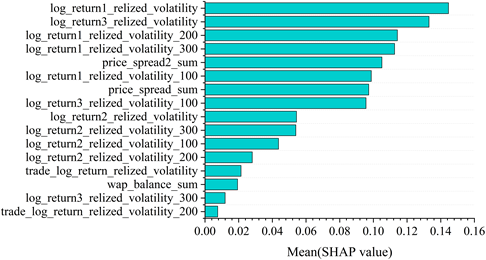
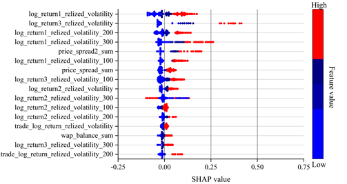
Boruta SHAP works based on the theory of Shapley value, which is a measure of how much each feature contributes to the prediction result. Its core idea is to distribute the contribution of each feature in proportion to its share of all possible combinations of features. In this way the total contribution of each feature to the prediction result is calculated and finally the average of the Shapley values of each feature is used as the SHAP value of that feature for feature selection. The results of the importance ranking of feature selection based on Shapley value for financial high frequency trading data are shown in Figure 1 and Figure 2.

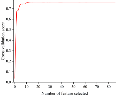
It can be seen from the figures that realized volatility and bid-ask spreads in different time windows have a greater impact on financial high frequency trading data. Based on the Shap value after ranking the importance of features, the features are brought into the model for training in descending order and 12 features are identified as the optimal feature subset.

3.3.1. Recursive feature elimination method feature selection

. Recursive Feature Elimination (RFE) is a wraparound feature selection method. A step-by-step feature removal method is adopted, starting from the least important feature, continuously removing a feature and retraining the model. After each training of the model, RFE ranks the features based on the model performance and then removes the lowest ranked feature. Figure 3 depicts the relationship curve between the number of features and model cross-validation. 10 most influential features were selected from the dataset as the optimal feature subset using RFE model cross-validation, and the most influential features in the feature subset were the weighted average price summation as well as the standard deviation, followed by realized volatility in different intervals and statistical features related to the bid-ask spread.

3.3.2. Analysis of the results of comparative experiments

. In order to validate the feature selection algorithm in this paper, experimental comparisons are made using Random Forest, Mutual Information, Shap and RFE feature recursive elimination methods, and each feature selection method is ranked in terms of feature importance, and then the feature data are brought into the LGBM neural network to perform cross iteration, with 70% of the data serving as the training set, and 30% of the data serving as the test set. The effect of different feature selection methods in volatility prediction of financial high-frequency trading data is compared through experiments, and the specific experimental results are shown in Table 1.

Table 1 Prediction effect comparison of feature selection methods

Feature selection method	Characteristic quantity	R2	RMSPE	MAE
Random Forest	39	0.782	0.257	7.17E-04
Mutual trust	35	0.741	0.271	7.38E-04
Shap	19	0.738	0.234	7.08E-04
RFE	16	0.740	0.255	6.99E-04
Ours	31	0.805	0.242	6.36E-04

According to the experimental results, it can be seen that the optimal feature subset selected from the financial high-frequency trading data features by Boruta SHAP algorithm used in this paper achieves a better prediction effect with RMSPE=0.242, which is better than other feature selection algorithms.

4. AMP-LSTM financial market volatility prediction model construction and testing

4.1. LSTM model of the benchmark

LSTM is a special type of RNN that maintains long-term information about the sequence. Due to this feature, LSTM has achieved great success in time series prediction.RNN can only use information that is very close to the relevant location to memorize and use for prediction, when the location of the two information is far away from each other, then the RNN will lose its learning ability. In addition, RNNs often cause gradient disappearance or gradient explosion during training. LSTM solves these problems by introducing a “gate” structure to selectively add or remove information to the memory storage unit. Valves are used between layers to control whether or not data is input, and how much data is input. A complete LSTM neuron contains one memory storage unit and three gating units, which are forgetting gate, input gate and output gate [26].

1) Forgetting gate. The oblivion gate mainly controls those information to be discarded from the memory storage unit. When the oblivion gate reads the output information $h_{t-1}$ of the previous module and the input information $x_t$ of the current period, it determines the amount of information that has passed through the sigmoid layer and passes that value to the number in each memory storage unit $c_{t-1}$. The formula for this is: $$\begin{array}{}\text{(6)}& f_t=\sigma (W_f\cdot [h_{t-1},x_t]+b_f),\end{array}$$ where $w_f$ denotes the weight matrix of the forgetting gate, and $b_f$ denotes the bias term of the forgetting gate, which is the parameter to be learned during the training process of the model, the same below.

2) Input gate. The input gate is mainly to control the new input information that needs to be stored in the memory storage unit. The sigmoid layer is used to decide the updated information $i_t$, then the tanh layer is used to create the candidate vector ${\tilde{C}}_t$, and finally the two information are multiplied to produce the updated state. The formula is as follows: $$\begin{array}{}\text{(7)}& i_t=\sigma (W_i\cdot [h_{t-1},x_t]+b_i),\end{array}$$ $$\begin{array}{}\text{(8)}& {\tilde{C}}_t=\mathrm{t}\mathrm{a}\mathrm{n}\mathrm{h}(W_C\cdot [h_{t-1},x_t]+b_C).\end{array}$$

3) Storage Memory Unit. To update the state of the storage memory cell from $c_{t-1}$ to $c_t$, first multiply the old storage memory cell state $c_{t-1}$ by $f_t$, discard the information that is determined to be discarded by the forgetting gate calculation, and then add the value of the product of the input gate information $i_t$ and the updated state ${\tilde{C}}_t$. The formula for this is: $$\begin{array}{}\text{(9)}& C_t=f_t\circ C_{t-1}+i_t\circ {\tilde{C}}_t,\end{array}$$ where “$\circ$” indicates multiplication by elements.

4) Output Gate. In the output gate is mainly to control the information after filtering to determine the value of the output. The output process is first through a sigmoid layer to determine which information can be output, and then through the above calculation of the state of the storage memory unit through the tanh processing is converted to (-1, +1) between the value of the value and the output gate information is multiplied by the final output of the information after the calculation to determine the need to output information. Its calculation formula can be expressed as: $$\begin{array}{}\text{(10)}& o_t=\sigma (W_o\cdot [h_{t-1},x_t]+b_o),\end{array}$$ $$\begin{array}{}\text{(11)}& h_t=o_t{}^{\circ }tanh(C_t).\end{array}$$

4.2. AMP-LSTM predictive modeling constructs

4.2.1. Structure of the AMP-LSTM

.

The AMP-LSTM consists of several layers and its structure is shown in Figure 4.

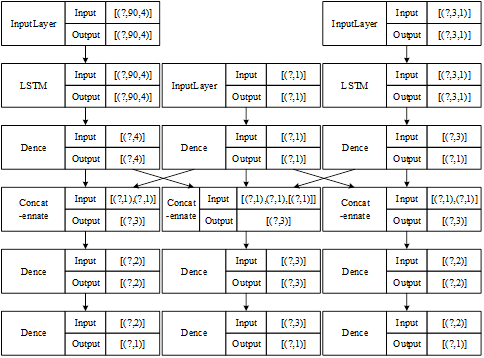
One is the input layer, which is used to construct the input of data. Since there are three different frequencies of data in this paper, the data with different frequencies are input in three input layers using the principle of setting time gates as described above. The time period of the daily data is set to 30, and since there are four short-term factor indices, the data dimension of this layer is 4. Setting a variable to indicate the use of data for the months of the quarter with a value in the range of [1, 2, 3] indicates that it is entered by 30, 60, 90, and then setting a lag variable with a value of $[1,2,3,\cdots ,n]$ for the lag variable, the number of days lagged is $30\times n$. Setting the period of the monthly data to 3, there is only one long term factor index in this paper therefore the dimension is 1. Sharing the above variables allows for the entry of 1, 2, and 3 months of data, representing the first month of the quarter, the first two months, and all 3 months of the quarter. The simultaneous sharing of the above lagged variables indicates that data lagged by multiple months can be added to the mix. For the lagged data of GDP growth rate, the data lagged by 1 period is used. The problem of inputting asynchronous mixing data is solved by controlling the data input at the three input layers described above.

The second is to set the Dropout layer, in order to prevent the model from overfitting phenomenon, the dropout layer is added to determine the discard rate of each layer of network nodes, the parameter size can be set according to the model fitting situation, its default value is 0.2, and the parameters are tuned in the process of model training and testing.

The third is the LSTM layer, where the input data is put into neurons for training according to fixed unit settings to extract the features of the data. This layer is mainly required to set the activation function used, the number of layers using LSTM, the number of hidden neurons contained in each layer, the use of regularization parameters, etc.

Fourthly, the connectivity layer is used to link the output data from the various data training mentioned above. And to integrate the data for output.

Fifth is the fully connected layer, which is used to control the output of the model, and the activation function can be set as well. In general, the system defaults the activation function of the output layer to a linear function. In the first fully connected layer is mainly to integrate the data, and the second layer uses the linear function to output the final result.

After completing the step of forward computation, the last is to use the compilation layer to optimize the computation results through error back propagation. In this layer it is necessary to set the way of calculating the error and the selection of the optimization method. By default the mean square error (MSE) is used as the loss function calculation method and the optimizer defaults to the optimization algorithm as Adam.

4.2.2. Hyperparameters of the model.

1) Activation function. The main role of the activation function is to give the model the ability to model nonlinearly. Traditional econometric models usually can only predict data through linear functions, but the activation function of LSTM can learn and understand complex nonlinear data features. When the input data is obtained as a new set of vectors through weighting and bias terms, it is by setting the activation function that the nonlinear features of the model expression are enhanced, thus extending the model to applications with nonlinear data. If the activation function is not set, the multiple layers of the LSTM setup merely multiply the data matrices of the layers to transform the input data into a linear combination of outputs. Therefore, in order to make the LSTM model fit the nonlinear data better, setting the activation function so that it arbitrarily approximates its nonlinear function can achieve better prediction results.

Common activation functions are segmented linear functions and nonlinear functions with exponential shapes in two categories, including sigmoid, tanh, ReLU, P-ReLU, Leaky-ReLU, etc. In this paper, we will comprehensively determine the form of the activation function according to the characteristics of each activation function, combined with the effect of model training.

2) Loss function. The established LSTM model needs two parameters to be set when compiling, one is the objective function setting and the other is the optimizer selection. One of the objective function is the loss function, which is used to calculate the error between the true value and the predicted value, and the model is corrected by the propagation of the calculated loss direction. Commonly used loss functions are mean square error (MSE), mean absolute error (MAE), mean absolute percentage error (MAPE) and so on. In this paper, MSE is used as the loss function to calculate the loss.

3) Optimization method. Another parameter that needs to be set in the compilation process of the model is the selection of the optimizer. Different optimizers correspond to different optimization methods, which are used to control the gradient descent, and update the corresponding parameters by back-propagating the gradient descent.

Subsequently, choosing a relatively reasonable optimization method for different data features and models can improve the performance of the model. Combining the characteristics of the data and the structure of the AMP-LSTM model in this paper, the Adam optimization method is chosen to control the gradient descent in the model compilation process.

4.3. Analysis of examples

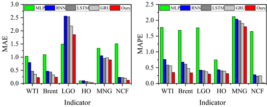
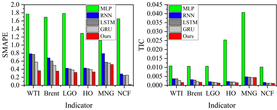
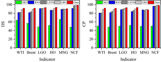
Six error class evaluation statistics such as Mean Absolute Error (MAE), Mean Absolute Percentage Error (MAPE), Terrell’s Inequality Coefficient (TIC) and Symmetric Mean Absolute Percentage Error (SMAPE), Directional Symmetry (DS) and Corrected Uptrend (CP) are used to evaluate the prediction performance of the model.The smaller the values of MAE, MAPE, SMAPE, and TIC, the larger the values of DS and CP values, the smaller the predicted and actual values are in terms of error and the closer they are in terms of directional trend, the better the predictive performance.

In order to better test whether the prediction results of the AMP-LSTM model are significantly different from those of the LSTM model, two hypothesis tests, t-test and W-rank-sum test, are chosen in this section. Table 2 shows the significance tests of the predicted results of the LSTM and AMP-LSTM models. The two-tailed test p-values for both methods are very close to 0, much less than the significance level of 0.05, and the H-values calculated by hypothesis testing are all 1, indicating that the test rejects the null hypothesis. In Table 2, t denotes t-test and W denotes Wilcoxon signed rank test. Therefore, the predicted results of the AMP-LSTM model are significantly different from the predicted values of the LSTM model. From the evaluation indexes and the parameter values of the fitted curves, the prediction effect of the AMP-LSTM is significantly better than that of the LSTM.The AMP-LSTM model improves the accuracy of the LSTM model in predicting the volatility of energy futures.

Table 2 Significance test of predictive error for LSTM and AMP-LSTM models

		WTI	Brent	LGO	HO	MNG	NCF
t	H	1	1	1	1	1	1
	T value	-0.0485	0.0358	0.0885	-0.0045	-0.0838	0.0228
	p	0	0	0	0	0	0
W	H	1	1	1	1	1	1
	T value	-18.9254	10.2785	23.2768	-2.1378	-26.8464	-7.0338
	p	0	0	0	0	0	0

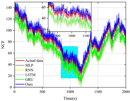
The model proposed in this paper is compared with LSTM model and other reference models (MLP, RNN and GRU) and the prediction results of these models are plotted in the same figure for comparison. Figures 5 to 9 show the prediction results of different models for six sets of energy futures indices. As can be seen from the enlarged subplots in the figures, the predicted values of the AMP-LSTM model are closest to the actual values. In addition, the values of MAE, MAPE, SMAPE and TIC of WTI predicted by the AMP-LSTM model are 0.2267, 0.2982, 0.3638 and 0.0021 by the values of the error-type evaluation index and the trend-type statistics index, respectively, which are smaller than the other comparative models.The values of DS and CP are 92.0000 and 92.8637, which are both greater than the other comparison models.

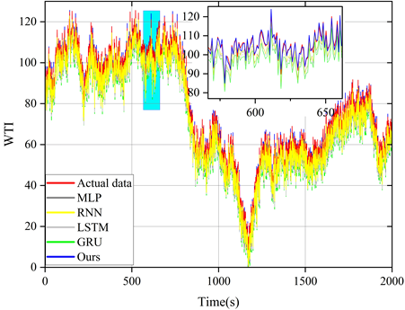
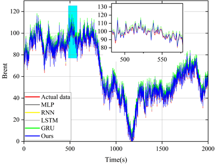
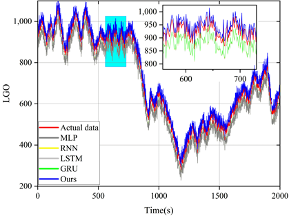
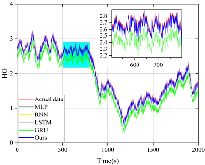
Through several iterations of experiments on these indicator values, the final average indicator values are displayed in the bar charts from Figure 10 to Figure 12. In general, the smaller the values of MAE, MAPE, SMAPE and TIC, and the larger the values of DS and CP, the better the prediction of the model. Therefore, the AMP-LSTM model outperforms other comparative models in terms of both error and trend.

In order to further assess the forecasting performance of the prediction models on the short-term volatility data of the energy futures indices, we forecasted and analyzed the annual 1-month and 3-month data of WTI and Brent crude oil futures indices using the evaluation metrics to compute their average MAPE values, and Table 3 shows the MAPE values of the various models of one month and three months for WTI and Brent. In Table 3, the minimum value of MAPE is 0.321 for 1 month and 0.346 for 3 months, which is still greater than the average MAPE for 6 months, 1 year and 8 years. If an extreme event occurs within this short period of time, the data set will be affected not only by other micro and macro factors, but also by this extreme event, which is very unstable and does not have a strong correlation with the subsequent predictions. Therefore, it can be seen that short-term fluctuations are not predicted as well as long-term fluctuations. However, since short-term volatility data is affected by more factors, the input variables of the model are not only the closing price, but also other variables, which enables the model to take more factors affecting the prediction results into account in the model training process to make the model’s prediction performance more accurate. From Table 3, it can be seen that the 1-month and 3-month average MAPE values in the AMP-LSTM model are still smaller than some of the long-term volatility predictions of the other models. Brent is the same way. Therefore, the short-term prediction of the AMP-LSTM model is also relatively good.

Table 3 MAPE value of various models of 1 and 3 months for WTI and Brent

Model	2016	2017	2018	2019	2020	2021	2022	2023	Average
WTI	One month
MLP	2.171	2.428	2.328	2.379	2.866	2.680	2.720	3.024	2.600
RNN	0.867	1.330	1.273	0.889	1.076	1.078	0.935	1.021	1.149
LSTM	0.920	0.949	0.810	0.752	0.675	0.727	0.701	0.669	0.785
GRU	0.640	0.851	0.809	0.407	0.743	0.851	0.817	0.702	0.736
AMP-LSTM	0.321	0.435	0.410	0.594	0.442	0.597	0.433	0.375	0.467
	Three months
MLP	2.110	2.225	2.134	1.945	3.057	2.526	2.093	2.660	2.258
RNN	1.027	1.026	0.891	0.937	0.886	0.856	1.016	0.407	0.735
LSTM	0.681	0.519	0.473	0.785	0.466	0.619	0.626	0.516	0.663
GRU	0.757	0.476	0.727	0.441	0.698	0.750	0.781	0.595	0.779
AMP-LSTM	0.346	0.367	0.577	0.174	0.317	0.566	0.441	0.261	0.201
Brent	One month
MLP	3.984	4.050	1.615	1.411	3.642	2.327	2.175	3.004	2.849
RNN	2.004	1.580	1.192	0.648	1.862	1.862	2.028	1.409	1.471
LSTM	1.103	1.304	0.536	0.561	1.498	1.228	1.636	1.480	1.382
GRU	0.666	0.755	0.623	0.412	0.850	1.322	1.165	0.865	0.897
AMP-LSTM	0.413	0.611	0.463	0.476	0.677	0.661	0.542	0.497	0.652
	Three months
MLP	2.849	2.372	1.484	1.613	2.719	2.412	2.049	2.412	2.131
RNN	0.619	1.207	0.282	0.461	1.382	1.285	1.765	1.290	1.147
LSTM	0.574	1.094	0.522	0.662	1.181	1.118	1.410	0.930	0.930
GRU	0.541	0.636	0.412	0.547	0.810	0.713	0.557	0.514	0.636
AMP-LSTM	0.373	0.444	0.285	0.311	0.523	0.564	0.699	0.485	0.513

Linear fitting of the various forecasting models reveals that the new model has a better fit. Table 4 shows the values of the linear regression parameters for the energy futures price index, and the a-value and R-value of the AMP-LSTM model for WTI are 1.011 and 1.005, respectively, which are closer to 1 than any of the other compared models. Therefore, the AMP-LSTM model has the best prediction performance.

Table 4 Linear regression parameter values of energy futures price indexes

	WTI			Brent			LGO
	a	b	R	a	b	R	a	b	R
MLP	1.267	-8.086	0.955	1.233	-6.895	1.014	1.192	36.406	1.034
RNN	0.951	1.710	0.996	0.907	1.933	0.994	0.989	13.264	1.002
LSTM	0.973	0.626	1.021	1.002	0.983	1.030	0.973	6.540	0.989
GRU	0.939	0.865	1.013	0.964	0.052	1.003	0.980	-1.071	0.978
AMP-LSTM	1.011	-0.063	1.005	0.999	-0.126	0.989	0.978	5.012	1.021
	WTI			Brent			LGO
	a	b	R	a	b	R	a	b	R
MLP	0.899	0.031	0.997	0.506	98.578	0.995	1.251	-8.286	0.989
RNN	1.019	0.097	1.050	0.989	4.146	0.996	0.957	0.471	1.008
LSTM	0.973	-0.004	1.013	0.997	-0.191	1.016	1.007	0.562	1.012
GRU	0.965	0.023	1.009	1.019	-0.534	0.998	1.067	-1.722	1.018
AMP-LSTM	1.010	0.006	1.000	0.990	0.969	1.011	1.027	0.047	0.984

5. Conclusion

This paper combines the Boruta and SHAP algorithms to model and characterize financial data, and constructs the AMP-LSTM model to learn and predict financial market volatility. Based on the experimental comparison of Random Forest, Mutual Information, Shap and RFE feature recursive elimination methods, the RMSPE value of Boruta SHAP algorithm used in this paper is 0.242, which is better than the other comparison algorithms and shows better prediction effect. The t-test results showed that the predictions of the AMP-LSTM model were significantly better (p$<$0.01) than the predicted values of the LSTM model. Compared to reference models such as MLP, RNN and GRU, the predicted values of the AMP-LSTM model are closest to the actual values. The MAE, MAPE, SMAPE and TIC values of WTI predicted by the AMP-LSTM model are 0.2267, 0.2982, 0.3638 and 0.0021, respectively, which are smaller than the other comparison models. It can be seen that the method in this paper has a more accurate forecasting performance in predicting financial market volatility.