
With the continuous progress of information technology, university library management is facing the urgent need to transform from the traditional mode to digitalization and intelligence. The traditional way of library management has the problems of low query efficiency, cumbersome borrowing and reading process, and low utilization rate of library resources, which is difficult to meet the actual needs of teachers and students. Therefore, it is particularly important to design and implement a system that integrates book management and personalized recommendation functions. The system aims to improve the efficiency of book management and optimize the borrowing process through information technology, and at the same time, provide readers with personalized book recommendation services to enhance the reading experience of readers [10, 17, 3].
Intelligent book recommendation system is a system that selects the books that users are interested in from a large number of digital book resources and recommends them to users by using various information such as users’ historical information and borrowing behavior. The purpose is to provide users with better book recommendation services, so that the user experience is more efficient and convenient [4, 6, 5]. Intelligent book recommendation system can be based on the user’s borrowing, reading habits, push the relevant books, to facilitate the user to find interesting books. In addition, the system can also sort the books according to the theme, classification, book reviews, etc., to provide users with more choices. Intelligent book recommendation system uses various algorithms such as intelligent machine learning, data mining technology, etc., so that it can accurately select the books that meet the user’s needs and improve the accuracy of book recommendation [13, 12].
[20] recommended books to readers using association rule mining models. The borrowing patterns of patrons are analyzed in order to improve the utilization of library resources. It is found that based on the analysis of readers’ borrowing patterns, it can realize the recommendation of books that may be interested to readers. Its shortcomings and improvement measures are also pointed out. [11] proposed an item-based collaborative filtering recommendation algorithm and developed an improved collaborative filtering algorithm by combining it with a user-based collaborative filtering recommendation algorithm. The results show that the proposed personalized intelligent book recommendation system for libraries has many advantages, such as high coverage and high accuracy, and can provide readers with more accurate and personalized recommendation services. [16] introduced an intelligent library personalized information service system based on multimedia network technology. The effectiveness of the system is proved through experiments, and its average absolute deviation is small, comprehensive performance is strong, and it plays an important role in improving work efficiency. [15] designed a personalized recommendation system for college libraries based on hybrid recommendation algorithm. Comparative experiments were carried out using hybrid algorithms on a dataset of a university library. The results emphasize that the hybrid approach can provide more accurate recommendations than the pure approach. And a personalized book recommendation system was successfully designed based on the combination of Spark big data platform and hybrid recommendation algorithm. [22] introduced user preferences into digital library recommender systems for personalized recommendations. The LDA model is utilized to estimate the topics, and the effectiveness of the intelligent library recommender system based on user preferences is verified based on experiments in a university digital library. [19] launched a systematic introduction to the intelligent discovery system, and studied its components, construction, etc., and examined the implementation strategy of the intelligent discovery system based on knowledge recommendation, with a view to providing a reference for the innovation and development of intelligent library service mode.
[24] introduced the architecture and key technologies of loT technology, as well as the definition and characteristics of regional library consortia and content. Measures such as establishing an information resource sharing organization and securing the information resource sharing security of regional library alliance are proposed. [18] designed the framework of library book recommendation system. By adopting readers’ borrowing records, combined with collaborative filtering model, thus selecting recommended books. It was emphasized that book recommendation service is beneficial to help users improve their reading interest and experience. [8] discussed personalized recommendation in libraries, points out the deficiencies of traditional libraries, and emphasizes that library users are subdivided into new users and ordinary users, and provides personalized reading services for different types of users based on big data. [2] developed an intelligent recommendation algorithm based on association rules and CF technology based on various problems exposed by digital libraries. And the effectiveness of the system was verified in experiments, which not only improved the utilization of digital books, but also reduced the retrieval time. [21] examined the personalized recommendation method of CFA-based intelligent book recommendation system for libraries by taking readers’ reading data and library bibliographic recommendation strategies as research objects. Through experiments, it was shown that the recommendation time of CFA optimized based on Kmeans algorithm was faster compared to the traditional CFA. [14] proposed the hybrid CFR, which aims to improve the recommendation service in university libraries. The hybrid recommender system combines content-based filtering and user-based collaborative filtering as well as clustering algorithms. Based on comparative experiments, the hybrid recommender system is proved to have very high recommendation accuracy. [23] discussed the design of a Java-based book query system, aiming to reduce the work pressure of library managers, thus improving the utilization of book resources and readers’ experience.
This paper designs personalized information recommendation model for intelligent library. Firstly, the label system of user portrait composed of basic information labels and behavioral information labels is set, and the label weights are set, and then the cluster user portrait model is visualized and analyzed by factor analysis and K-means clustering algorithm. Then the basic concepts and related formulas such as intelligent body, value function and strategy iteration in reinforcement learning are modeled, and optimization and improvement are carried out on the basis of Actor-Critic framework, which, in the Actor model, utilizes the Transformer deep neural network training parameter, outputs a list of recommended items obtained based on the current state, and uses it as the Critic’s Input. Meanwhile, in the Critic model, the EDQN network structure is used and the same Transformer deep neural network as in Actor is employed. After conducting performance tests on the dataset and exploring the effects of important parameters, the model is applied to real recommendations.
Labeling of user information is a prerequisite for the construction of a library user portrait model centered on user needs, which requires the design of a labeling system that comprehensively reflects user data and information, as well as the setting of the size of the labeling weight in accordance with the reality, so that the library’s personalized recommender service can achieve real differentiation and intelligence.
This paper is based on the research results related to the construction of the domestic user image model, combined with the actual situation of the library user image, the library user image model is divided into data collection layer, data processing layer and data application layer (Figure 1).
(1) Data acquisition layer. Data collection is the basis for building a user profile model, and the collected data mainly includes user static data and dynamic data. In this paper, we collect static data such as name, gender, user ID number, book information borrowed by the user, etc. Meanwhile, we also collect dynamic data generated when users interact with libraries, i.e., the user’s borrowing content, borrowing time, return status, purchasing records, etc., reflecting the user’s borrowing preference dynamic information.
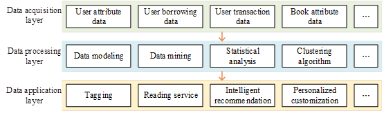
(2) Data processing layer. The processing of data is a key step in building a user profile model. Generally speaking, the collected data can not be directly used to create a user profile model, but to be manually cleaned and screened according to the actual state of the research, remove invalid information, retain valuable data and supplement the missing data, and then use mathematical algorithms or computer technology to process the data, so that the complicated data symbols into a standardized data text, to provide the basis for the application of the user profile model and to assist enterprises to scientific decision-making.
(3) Data application layer. Data application is the ultimate purpose of building a user profile model. It is directly oriented to the majority of user groups, and services such as smart recommendation and personalized customization play a positive and significant role in improving the quality of library services. After the data processing process, the user’s interest preferences at a specific time and situation are labeled, and users with high interest relevance or similarity are clustered into a group or a cluster to refine user characteristics. In this way, the system can accurately identify user labels, depict user profiles, and provide users with a series of intelligent and actively responsive personalized recommendation services according to their own needs.
User portrait labels are designed according to the characteristics of collected user data, and the completeness of the labeling system will affect the accuracy of the portrait. In this paper, the types of library user portrait labels are divided into basic information labels and behavioral information labels.
The user’s basic information label is the user’s relatively stable information, which is the most basic part of the user image, including name, gender, user ID, book information borrowed by the user, and other static information, which can be extracted directly without too much testing work.
The user’s behavioral information label is an important basis for reflecting the user’s interests and preferences as well as the interaction process, this paper will collect the behavioral information of the library user data, which mainly includes the user’s borrowing content, borrowing time, return status, purchase records, and other dynamic information that can reflect the user’s borrowing preferences to a certain extent.
For different types of service platforms in the market, in order to build a user profile that highly matches the nature of the platform, the design of the labeling system should be in line with the platform’s usage scenarios, functional requirements and development goals. In this paper, after fully considering the library application scenario, information collection cost, privacy and security elements, the user labeling system constructed is mainly for the following three aspects: First, the basic information, including name, contact information, user ID, the user’s borrowed book information (the title of the book, the author of the book, the type of the book) and so on. The second is behavioral information, including borrowing content, borrowing time, return status, purchase time, number of purchases, transaction amount and other information reflecting user preferences.
The label represents the user’s point of interest, and the label weight indicates the user’s degree of preference. According to the user’s actual borrowing behavior, this chapter divides the dimensions of user portrait into user basic information dimension and behavioral information dimension, and extracts representative data features according to the different dimensions where the data are located. According to the classification of the Chinese Library Classification, and drawing on Douban’s classification of book themes, and combining with the actual borrowing situation of libraries, a total of 25 reading themes are categorized, including poems and prose, literature (fairy tales and fables, sociology, etc.), history, music, travel, food, art, life (parenting, sports and fitness, life attitudes, etc.), reasoning and suspense, gender, emotions, inspirational, healing, science fiction, magic, war, fiction, novels, and other topics. , Magic, War, Fiction, Growth, Psychology, Popular Science, Teaching Aids, Economy, Faith, Miscellaneous Writings, Philosophy. Each topic word is used as a label under the dimension of user behavioral information, and the frequency of occurrence is counted, and the frequency of counting is set as the weight of the label, and the higher the frequency, the higher the weight value of the label, the higher the degree of user preference.
After screening and cleaning the collected library user data, the portrait model is built with the help of machine learning, neural network, data mining and other technologies, relying on Bayesian function, decision tree, clustering algorithm and so on. In order to comprehensively understand user characteristics, this paper first uses factor analysis to statistically analyze user data, and then builds a library user portrait model through clustering algorithm. User portrait clustering is a common method for classifying user characteristics, using the degree of similarity between the user and the user characteristics, the high degree of similarity of the user clustered into a group, that is, the group user portrait, the group of users within the user’s characteristics or attributes are similar or similar, while the user characteristics between the groups are more different.
(1) Factor analysis. Assume that there is \(n\) sample and \(p\) indicators (with strong correlation between indicators) are observed for each sample. To facilitate the study, the sample data need to be standardized, is standardized variable mean 0, variance 1. For convenience, both the original variables and the standardized variable vector are denoted by \(X\), with \(F_{1} ,F_{2} ,\ldots ,F_{m} (m<p)\) denoting the standardized common factor. If:
(1) \(X=(X_{1} ,X_{2} ,…,X_{p} )^{{'} }\) is an observable random vector with mean vector \(E(X)=0\), covariance matrix \(cov(X)=\Sigma\), and covariance matrix \(\Sigma\) is equal to correlation matrix \(R\).
(2) \(F=(F_{1} ,F_{2} ,…,F_{m} )^{{'} } (m<p)\) is an unobservable variable with mean vector \(E(F)=0\), covariance matrix \(cov(F)=I\), i.e., the components of vector F are independent of each other.
(3) \(\varepsilon =(\varepsilon _{1} ,\varepsilon _{2} ,\ldots ,\varepsilon _{p} )^{{'} }\) is independent of F and the covariance matrix \(\Sigma _{\varepsilon }\) of \(E(\varepsilon )=0\), \(\varepsilon\) is diagonal square: \[\label{GrindEQ__1_} {\rm cov}(\varepsilon )=\Sigma _{\varepsilon } =\left[\begin{array}{cccc} {\sigma _{11} {}^{2} } & {} & {} & {0} \\ {} & {\sigma _{22} {}^{2} } & {} & {} \\ {} & {} & {\ddots } & {} \\ {0} & {} & {} & {\sigma _{pp} {}^{2} } \end{array}\right] . \tag{1}\]
That is, the components are also independent of each other. Then the model: \[\label{GrindEQ__2_} \left\{\begin{array}{c} {X_{1} =a_{11} F_{1} +a_{12} F_{2} +\cdots +a_{1m} F_{m} +\varepsilon _{1} } ,\\ {X_{2} =a_{21} F_{1} +a_{22} F_{2} +\cdots +a_{2m} F_{m} +\varepsilon _{2} }, \\ {\vdots } \\ {X_{p} =a_{p1} F_{1} +a_{p2} F_{2} +\cdots +a_{pm} F_{m} +\varepsilon _{p} }. \end{array}\right. \tag{2}\]
It is called factor model.
(2) K-means clustering algorithm. The K-means algorithm is the classic division-based clustering algorithm. Using the sample distance as a division criterion, the sample distance is inversely related to the sample similarity, i.e. the smaller the distance between two samples, the higher the similarity; the larger the distance, the smaller the similarity [1]. The algorithm generally uses the Euclidean distance to calculate the distance between the samples, the formula is as follows: \[\label{GrindEQ__3_} d(x,y)=\sqrt{\sum _{i=1}^{n}(x_{i} -y_{i} )^{2} } , \tag{3}\] where \(x_{i}\) is the \(i\)nd sample object, \(y_{i}\) is the \(i\)th clustering center, and \(n\) is the dimension of the sample object.
During the clustering process, the class center, which is the average of all samples in the class, needs to be recalculated at each iteration.
Assuming that the class center of the \(\; k\)th class is \(Center_{k}\), the updated \(Center_{k}\) is calculated as follows: \[\label{GrindEQ__4_} Center_{k} =\frac{1}{|c_{k} |} \sum _{x_{i} \in c_{k} }x_{i} . \tag{4}\]
The clustering algorithm requires constant iterations to reclassify the categories and update \(Center_{k}\), and the iteration ends when the termination condition is met. The termination condition is generally set to reach the maximum number of iterations or the objective function is less than a threshold. The objective function is: \[\label{GrindEQ__5_} J=\sum _{k=1}^{K}\sum _{x_{i} \in c_{k} }d (x_{i} ,Center_{k} ) . \tag{5}\]
Reinforcement learning focuses on the problem of how to maximize rewards from the environment. Among them, the algorithm part is called the intelligent body, as shown in Figure 2, the intelligent body acquires the environment state \(S_{t}\), and after the algorithm calculates and outputs an action \(A_{t}\), after the environment receives the action \(A_{t}\), it will give a feedback to the intelligent body \(R_{t}\), and produces the next state \(S_{t+1}\), which continues to be infused into the intelligent body, and so on and so forth, and this is the most basic reinforcement learning model. Reinforcement learning uses exploration to gain an understanding of the environment, and then uses that knowledge to gain greater rewards.
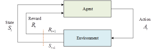
An intelligent body interacts with its environment, which gives it feedback signals called rewards, denoted by \(R\). The ultimate goal of the intelligent body is to maximize the cumulative rewards over its entire life cycle. Rewards in the environment are delayed, i.e., the reward at moment \(t\) is not only associated with the action at moment \(t\), but with all actions up to moment \(t\), so that the intelligent body can learn longer-term feedback. The set of all valid actions in a given environment is called the action space, denoted by \({\rm {\mathcal A}}\), e.g., in Go the action space is all the positions on the board where a move can be made. If the number of actions is finite, it is a discrete action space, and if it is infinite, it is a continuous action space, and the actions in a continuous action space are generally real-valued quantities. Similarly, the space consisting of the states of the environment is called state space, denoted by \({\rm {\mathcal S}}\). For the intelligent body, the state of the environment can be regarded as the historical sequence of the intelligent body’s interaction with the whole environment. If \(o_{t}\) represents an observation of the environment by an intelligent body at the moment of \(t\), the sequence of interactions of the intelligent body with the environment can be expressed as follows: \[\label{GrindEQ__6_} H_{t} =o_{1} ,a_{1} ,r_{1} , o_{2} ,a_{2} ,r_{2} ,…o_{t} ,a_{t} ,r_{t} , \tag{6}\] and the state of the environment can be represented as a function of this historical sequence: \[\label{GrindEQ__7_} S_{t} =f(H_{t} ) . \tag{7}\]
Reinforcement learning algorithms simplify modeling by modeling the environment-intelligence interaction as a Markov decision model [9]. The Markov decision model assumes that the model has Markovianity, i.e., the state \(s_{t}\) at the current moment \(t\) is only related to \(s_{t-1}\) and is independent of all previous states: \[\label{GrindEQ__8_} p(s_{t+1} |s_{t} )=p(s_{t+1} |h_{t} )\quad h_{t} =\{ s_{1} ,s_{2} ,…,s_{t} \} . \tag{8}\]
Such a sequence of random variables with Markovian properties is a Markov process, and a discrete-time Markov process is said to be a Markov chain.
In reinforcement learning, Markov processes need to be combined with reward functions. The intelligence is rewarded in a round of interaction and defined as a reward, denoted as \(G_{t}\): \[\label{GrindEQ__9_} \begin{array}{rcl} {G{}_{t} } & {=} & {r_{t+1} +\gamma r_{t+2} +\gamma ^{2} r_{t+3} +…+\gamma ^{T-t-1} r_{T} } \\ {} \end{array} . \tag{9}\]
The value function for the current state is defined as the expectation of a return: \[\label{GrindEQ__10_} V^{t} (s)={\rm {\rm E}}[G_{t} |s_{t} =s] , \tag{10}\] where \(R(s)\) represents the immediate reward, \(s^{{'} }\) can be interpreted as the plenary state, and \(p(s^{{'} } |s)\) represents the probability of transferring from \(s\) to \(s^{{'} }\).
The Markov reward process also needs to be combined with the actions of the intelligences in order to constitute the final Markov decision process. Specifically, it is the transfer probability in the Markov reward process that has an additional condition: \[\label{GrindEQ__11_} p(s_{t+1} |s_{t} ,a_{t} )=p(s_{t+1} |h_{t} ,a_{t} ) . \tag{11}\]
Policy is an important concept in reinforcement learning, a policy defines the probability that an intelligent will take a certain action in a certain state: \[\label{GrindEQ__12_} \pi (a|s)=p(a_{t} =a|s_{t} =s) . \tag{12}\]
Similarly to the value function, the action value function, generally referred to as the Q-function, defines the expectation of the reward to be obtained by taking a certain action in a certain state, and here in this paper we directly give the Bellman equation form of the Q-function: \[\label{GrindEQ__13_} \begin{array}{rcl} {Q(s,a)} & {=} & {{\rm {\rm E}}[G_{t} |s_{t} =s,a_{t} =a]}, \\ {} & {=} & {R(s,a)+\gamma \sum _{s'\in S}p (s'|s,a)V(s')}. \end{array} \tag{13}\]
In the above equation, if all the actions are summed, the definition of the value function in the Markov decision process is obtained: \[\label{GrindEQ__14_} V(s)=\sum _{a\in A}\pi (a|s)Q(s,a) . \tag{14}\]
This equation represents the relationship between the value function, the strategy, and the Q function. The purpose of the reinforcement learning intelligences is to find the optimal strategy, or the optimal value function, which maximizes the final cumulative discount reward.
Depending on the iterative method, the iterative methods for intelligences can be categorized into two methods: strategy iteration and value iteration. In strategy iteration, the algorithm initializes a strategy \(\pi\), and makes it converge to the best strategy by continuously iterating this strategy. In strategy iteration, the first step is to evaluate the strategy \(\pi\), i.e., to compute the value function \(V_{\pi } (s)\). Here, in this paper, we directly give the value function based on Bellman’s equation: \[\label{GrindEQ__15_} V_{\pi } (s)=\sum _{a\in A}\pi (a|s)\sum _{s'\in S}p (s'|s,a)[R(s,a)+\gamma V_{\pi } (s')] . \tag{15}\]
By randomly initializing an initial value \(v_{0}\) and then iteratively updating it through the above equations, the algorithm is able to eventually obtain a sequence \(\{ v_{k} \}\) which, when \(k\to \infty\), is guaranteed to \(v_{k}\) converge to \(V_{\pi }\). By \(V_{\pi }\) being able to evaluate the goodness of a strategy, the algorithm is able to go further in search of a better strategy, a process called strategy boosting. The strategy boosting process is done by calculating the Q-function under the current strategy and then making the new strategy equal to the action that enables it to get the maximum value, i.e., \[\label{GrindEQ__16_} \pi _{k+1} (s)=\arg \max _{a} Q_{\pi ,k} (s,a) . \tag{16}\]
This strategy is greedy because it takes the next best strategy each time. The two means of strategy evaluation and strategy enhancement are defined above, and strategy iteration is the alternate use of strategy evaluation and strategy enhancement until the value function converges.
A disadvantage of policy iteration is that each policy evaluation process requires iterative computation over the entire set of states, and such an algorithm can only converge accurately in the end to \(V_{\pi }\). Real-world scenarios will most likely not require, and are unlikely to achieve, such an accurate optimal policy. The idea of value iteration, another learning method of reinforcement learning, is to stop the computation at one iteration for each policy evaluation. Value iteration can be understood as iterating directly through the Bellman equation: \[\label{GrindEQ__17_} Q_{k+1} (s,a)=R(s,a)+\gamma \sum _{s'\in S}p (s'|s,a)V_{k} (s') , \tag{17}\] \[\label{GrindEQ__18_} V_{k+1} (s)=\max _{a} Q_{k+1} (s,a) . \tag{18}\]
After iterating to the specified number of times \(H\), the optimal policy can be extracted as follows: \[\label{GrindEQ__19_} \pi (s)=\arg {\mathop{\max }\limits_{a}} \left[R(s,a)+\gamma \sum _{s'\in S}p (s'|s,a)V_{H+1} (s')\right] . \tag{19}\]
In applications of reinforcement learning, there is no perfect model of the environment in many scenarios, i.e., the complete Markov process model is not directly available in all the above formulas, and the transfer probability between one state and the next is not known. Therefore a method is needed to learn the strategy or value function without knowing the transfer probabilities. Monte Carlo sampling (MC) method is one of the learning methods, which learns the corresponding values by averaging multiple trajectories through learning trajectory data from reinforcement learning. Another method, and the most widely used method, is the temporal difference learning method (TD). The temporal difference method combines Monte Carlo and dynamic programming ideas, and instead of waiting until the end of the round to learn as in the Monte Carlo method, the fastest way to start learning is just at the next time step, i.e., every time the intelligent body interacts, it updates the value function of the previous moment with the reward it gets: \[\label{GrindEQ__20_} V(s_{t} )\leftarrow V(s_{t} )+\alpha (r_{t+1} +\gamma V(s_{t+1} )-V(s_{t} )) , \tag{20}\] where \(\delta _{t} =r_{t+1} +\gamma V(s_{t+1} )-V(S_{t} )\) is the TD error.
One of the biggest advantages of the temporal difference method is that it can be implemented in an online manner without waiting until the end of the round to update, especially in some scenarios where the rounds are very long, and if the learning is delayed until the end of the round, then it will lead to too slow learning efficiency. Therefore the learning model based on temporal difference methods is currently used in most reinforcement learning methods.
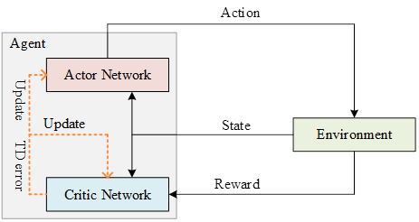
The structure of the Actor-Critic model is shown in Figure 3, where Actor is the strategy network for learning a strategy to get the highest reward, and Critic is the value network for evaluating how good the current strategy is. The earliest Actor-Critic algorithm was based on the strategy gradient, replacing the round reward in Eq. (21) with a Q function, and then updating it using TD-Error: \[\label{GrindEQ__21_} \nabla \bar{R}_{\theta } \approx \frac{1}{N} \sum _{n=1}^{N}\sum _{t=1}^{T_{n} }\left(r_{t}^{n} +V_{\pi } (s_{t+1} )-V_{\pi } (s_{t} )\right) \nabla \log \pi _{\theta } (a_{t}^{n} |s_{t}^{n} ) . \tag{21}\]
The use of deterministic strategies, while efficient in obtaining optimal actions, loses the stochastic nature of the model and leads to difficulties in exploration. A SoftActor-Critic (SAC) method was proposed by Haarnoja et al. The SAC algorithm proposes a model based on Maximum Entropy Reinforcement Learning (MERL), which optimizes the information entropy of the strategies while optimizing the strategies, i.e., to make the strategies as diverse as possible.The SAC method has an excellent performance in the field of robotics control, with high stability and robustness.
The aim of this paper is to validate the importance of list-based recommendations during user-agent interactions and to develop a new approach to incorporate them into the proposed list-based recommendation framework DAC-T [7].
Practical recommender systems typically suggest to each user an automatically generated list of product items that are tailored to the user’s preference profile. List-based recommendation item suggestions are preferred in practice because they allow the system to provide the user with a variety of complementary options. For list-based recommendations, we have a list-based operation space where each operation is a set of multiple interdependent sub-operations (items). Existing reinforcement learning recommendation methods can also recommend a list of items. For example, DQN can compute the Q-values of all recalled items separately and recommend a list of items with the highest Q-values. However, these methods recommend items based on the same state and ignore the relationship between recommended items. As a result, the recommended items are similar. In fact, bundling complementary items may yield higher returns than recommending all similar items. Therefore, in this paper, we generate a list of complementary items to improve performance by capturing the relationships between recommended items.
When we apply deep reinforcement learning to the problem under study, there are two main challenges: (1) large (even continuous) and dynamic action spaces (item spaces) and (2) the computational cost of choosing an optimal action. In practice, it is not enough to represent projects with discrete metrics, because we cannot learn from the metrics how different projects are related to each other. A common approach is to use additional information to represent items with continuous embedding. In addition, the behavior space of recommender systems is dynamic because items are arriving and departing. Moreover, computing the Q-values of all state-action pairs is very time-consuming due to the huge state space and action space.
To address these challenges, in this paper, our recommendation policy builds on the Actor-Critic framework, which is the preferred architecture from the point of view of the studied problem picking, as it is suitable for large and dynamic action spaces and also reduces redundant computations at the same time as compared to alternative architectures.
As mentioned above, we model the recommendation task as a Markov Decision Process (MDP) and utilize Reinforcement Learning (RL) in order to automatically learn the optimal recommendation strategy, which allows for continuous updating of the strategy during recommendation interactions and development of the optimal strategy. The user is rewarded by maximizing the expected long-term accumulation. Based on this, we formally define five elements of the tuple MDP \((S,A,P,R,\gamma )\) as follows:
(1) State space S: a state \(s\in {\rm {\mathcal S}}\) defined as the user’s current preference, whose generation is based on the user’s browsing history, i.e., the items that the user has browsed and her corresponding feedbacks; and a \(\; t\)-moment state \(s_{t} =\{ s_{t}^{1} ,…,s_{t}^{N} \} \in S\), defined by the first N items that the user has browsed.
(2) Action space A: a \(t\) moment of \(action{\rm \; }a_{t} =\{ a_{t}^{1} ,…,a_{t}^{K} \} \in A\), which is the K items recommended by RA based on the user’s current state \(\; s_{t}\).
(3) Reward R: After the RA takes \(action{\rm \; }a_{t}\) based on the current state \(s_{t}\), i.e., the page items are recommended to the user, who browses these items and provides his feedback. The user can issue actions such as click/skip, etc., and the model thus gets \(reward{\rm \; }r_{t} =r(s_{t} ,a_{t} )\).
(4) Transition probability P: The transition probability \(p(s_{t} +1|s_{t} ,a_{t} )\) defines the probability that the state changes from \(s_{t}\) to \(s_{t+1}\) after the RA takes \(action{\rm \; }a_{t}\). In particular, if the user does not take any action on M items recommended by \(action{\rm \; }a_{t}\), then \(s_{t+1} =s_{t}\), otherwise \(s_{t+1}\) will be obtained by \(s_{t}\) update.
(5) Discount factor \(\gamma :\gamma {\rm }[0,1]\), which mainly indicates the discount factor for measuring future rewards. In particular, when \(\gamma =0\), the recommendation agent will only consider immediate rewards. In other words, when \(\gamma =1\), all future rewards can be fully accounted for in the rewards of the current behavior, i.e., \({\rm cumulative\; reward}=r_{t} +\gamma r_{t+1} +\gamma ^{2} r_{t+2} +\cdots\).
An online environment simulator is built based on the user’s history, where the input is the current state and the action taken, and the output is the online reward computed by the simulation.Meanwhile, due to the huge space of items, which results in the vast majority of items not being in the user’s history, which poses a problem in calculating the reward, and the online environment simulator can exactly solve the above The online environment simulator solves these two problems.
Based on the above algorithm to create the cache \(M=\{ m_{1} ,m_{2} ,…\}\), at this point if we want to simulate the computation of the reward obtained from \(pair_{t} =(s_{t} ,a_{t} )\), then in turn will be \(pair_{t}\) and \(m_{i} =((s_{i} ,a_{i} )\to r_{i} )\) in \((s_{i} ,a_{i} )\) to calculate the cosine similarity, take the cosine similarity of the largest in the \(r_{i}\) will be the simulator to obtain the reward. \[\label{GrindEQ__22_} cos(pair_{t} ,m_{i} )=\alpha \frac{s_{t} s_{i}^{Transpose} }{||s_{t} ||||s_{i} ||} + (1-\alpha ) \frac{a_{t} a_{i}^{Transpose} }{||a_{t} ||||a_{i} ||} . \tag{22}\]
Before presenting the Actor model, we first need a brief introduction to Transformer. The vast majority of sequence processing models use an encoder-decoder structure, where the encoder maps an input sequence \((x_{1} ,x_{2} ,\ldots ,x_{n} )\) to a continuous representation \(\vec{z}=(z_{1} ,z_{2} ,\ldots …z_{n} )\), and then the decoder generates an output sequence \((y_{1} ,y_{2} ,…,y_{m} )\), outputting a result at each moment.The Transformer model continues this model, which is still essentially a model based on the mechanism of multiple attention.
The whole Transformer model is divided into two parts: encoder and decoder.
The encoder has N=6 layers and each layer includes two sub-layers:
(1) The first sub-layer is the multi-head attention mechanism, which is used to compute the input self-attention
(2) The second sub-layer is a simple fully connected network.
The decoder is also N=6 layers and each layer includes 3 sub-layers:
(1) The first one is the masked multi-head self-attention mechanism, that is, by calculating the self-attention of the input, but because of the lag in the generation process, the attention mechanism has no result for moments greater than \(t_{i}\) at moment \(t_{i}\), and only the self-attention mechanism before moment \(t_{i}\) has a result, so it needs to do the Mask operation.
(2) The second sub-layer is fully connected network, same as encoder.
(3) The third sub-layer is the attention computation on the input of the encoder.
The above defines status as the entire browsing history, which can be infinite and inefficient. A better approach would be to consider only active items. For example, the top 10 clicked/ordered items. A good recommender system should recommend the user’s favorite items. Positive items represent key information about user preferences, i.e., which items the user likes. Therefore, we only consider their state-specific scoring functions.
The Actor model can actually be viewed as a function: \[\label{GrindEQ__23_} f_{\theta ^{\pi } } :s_{t} \to w_{t} . \tag{23}\]
Transformer deep neural network is the computational process of the function, \(\theta ^{\pi }\) is the parameters of the function, the process of training Actor, in fact, is the process of constantly optimizing \(\theta ^{\pi }\) parameters.
The output \(w_{t}\) of the model is a weight factor for a scoring function, which is as follows: \[\label{GrindEQ__24_} score_{i} =w_{t}^{k} e_{i}^{T} . \tag{24}\]
The Critic model is used to calculate the Q value of the action sequence \(a_{t}\) generated by the Actor in state \(S_{t}\), and the parameters \(\theta ^{\pi }\) of the Actor can be updated based on the obtained Q value, where Q is calculated as follows: \[\label{GrindEQ__25_} Q*(s_{t} ,a_{t} ) =E_{s_{t+1} } [r_{t} +\gamma Q*(s_{t+1} ,a_{t+1} ) |s_{t} ,a_{t} ] . \tag{25}\]
In terms of the way of calculating Q-value, DQN has numerous advantages over Q-learning, so Critic chose to use DON for the implementation, and in order to capture more potential features, Critic’s DON network structure uses the same Transformer deep neural network as Actor.
The process of optimizing the Critic model is actually optimizing its parameter \(\theta ^{\mu }\). The loss function used in the optimization process is as follows: \[\label{GrindEQ__26_} L (\theta ^{\mu } ) =E_{s_{t} ,a_{t} ,r_{t} ,s_{t+1} } [ (y_{t} -Q (s_{t} ,a_{t} ;\theta ^{\mu } ) )^{2} ] , \tag{26}\] \[\label{GrindEQ__27_} y_{t} =E_{s_{t+1} } [r_{t} +\gamma Q^{{'} } (s_{t+1} ,a_{t+1} ;\theta ^{\mu ^{{'} } } ) |s_{t} ,a_{t} ] , \tag{27}\] and parameter optimization is performed using stochastic gradient descent based on this loss function.
DDPG is off-policy deep reinforcement learning algorithm based on Actor-Critic architecture. Let Actor be \(\mu (s;\theta ^{\mu } )\) and Critic be \(Q(s,a;\theta ^{0} )\), in order to compute the target behavior and target Q-value, let Actor target network \(\mu ^{{'} } (s;\theta ^{\mu {'} } )\) and Critic target network \(Q^{{'} } (s,a;\theta ^{Q{'} } )\). DDPG adds noise \(N\) to the Actor behavior to increase the exploration and produce a new behavior as: \[\label{GrindEQ__28_} \mu '(s_{t} )=\mu (s| \theta ^{\mu } )+N . \tag{28}\]
The critic network updates the network parameters by minimizing the loss function \(L(\theta ^{Q} )\) as: \[\label{GrindEQ__29_} L(\theta ^{Q} )=E_{s_{t} ,a_{t} ,r_{t} ,s_{t+1} } \left[(y-Q(s_{t} ,a_{t} | \theta ^{Q} ))^{2} \right] , \tag{29}\] \[\label{GrindEQ__30_} y=r(s_{t} ,a_{t} )+\gamma Q'(s_{t+1} , \mu '(s_{t+1} | \theta ^{\mu '} )| \theta ^{Q'} ) . \tag{30}\]
The actor network updates its parameters to: \[\label{GrindEQ__31_} \nabla _{\theta ^{\mu } } \mu |_{s_{i} } \approx \frac{1}{N} \sum _{i}Q (s,a| \theta ^{Q} )|_{s=s_{i} ,a=\mu (s_{i} )} \nabla _{\theta ^{\mu } } \mu (s| \theta ^{\mu } )|_{s_{i} } . \tag{31}\]
The Actor-Critic network in this chapter is updated in a different way than the DQN algorithm, where the target network is synchronized with the Q-network at intervals, whereas the weights of the Actor’s and Critic’s respective target networks in the DDPG’s strategy are added to the performance of the evaluations to be updated at a slower rate of change, but this approach also improves the stability of the learning process: \[\label{GrindEQ__32_} \theta ^{Q^{{'} } } =\tau \theta ^{Q} +(1-\tau )\theta ^{Q^{{'} } } , \tag{32}\] \[\label{GrindEQ__33_} \theta ^{\mu ^{{'} } } =\tau \theta ^{\mu } +(1-\tau )\theta ^{\mu ^{{'} } } . \tag{33}\]
In the above equations, \(\tau\) is the update factor and \(\tau \ll 1\), it is experimentally demonstrated that the DDPG remains stable across a range of action-space tasks.
In this section, experiments are launched on four real datasets to compare the performance of the proposed DRR with other state-of-the-art methods and to analyze the performance of the model under different experimental settings as well as to analyze the experimental results.
Popularity is a popularity-based method that recommends the most popular items to the user at a time, i.e., those with the highest average rating. According to the setting in the literature, the head few popular items with low number of ratings are removed.
PMF is a matrix decomposition method similar to SVD. It does matrix decomposition in the case of considering only non-zero elements to get the hidden vectors of users and items for recommendation.
SVD++ combines a matrix decomposition model and a nearest neighbor model to make recommendations.DeepFM explicitly models the interaction of low-order and high-order features to make recommendations.
AFM uses attention networks to explicitly learn the importance of feature interactions to make recommendations.
LinUCB makes recommendations by predicting an upper confidence bound on the potential reward of each item.
HLinUCB builds on LinUCB by further modeling the implicit features of each item to predict the potential reward of each item.
DQN uses a deep Q network to compute the Q-value of each action for the current state and recommends the item corresponding to the maximum Q-value to the user.
DDPG models the user state using a fully connected network and updates the model via a deep deterministic policy gradient algorithm, which serves as a baseline to compare the effectiveness of the user state representation module proposed in this chapter.
DEERS represents the user state by modeling the user’s positive and negative browsing history through recurrent neural networks respectively, and then does the recommendation under the deep Q-network architecture.
Table 1 shows the ranking results of each comparison model on the ML (1M) and Jester datasets. The model in this paper outperforms the rest of the models on both datasets for all observations, Precision@20 were 0.7174 and 0.3949, respectively.
| Model | ML(1M) Jester | Jester | ||||
| Precision@20 | NDCG@20 | MAP | Precision@20 | NDCG@20 | MAP | |
| Popularity | 0.5948 | 0.9098 | 0.618 | 0.3504 | 0.9125 | 0.4039 |
| PMF | 0.5957 | 0.9143 | 0.6684 | 0.3676 | 0.9191 | 0.4267 |
| SVD++ | 0.5998 | 0.9282 | 0.6612 | 0.3697 | 0.9046 | 0.4482 |
| AFM | 0.6606 | 0.9186 | 0.733 | 0.3744 | 0.9095 | 0.4617 |
| DeepFM | 0.6531 | 0.9258 | 0.742 | 0.3929 | 0.9186 | 0.4534 |
| DQN | 0.6238 | 0.9132 | 0.6963 | 0.3813 | 0.91 | 0.4536 |
| DDPG | 0.632 | 0.9172 | 0.6908 | 0.3731 | 0.9091 | 0.4445 |
| DEERS | 0.6774 | 0.9334 | 0.7524 | 0.3774 | 0.9188 | 0.4607 |
| This model | 0.7174* | 0.9359* | 0.7975* | 0.3949* | 0.9383* | 0.5053* |
The reasons for the observations can be analyzed from three aspects: (1) the proposed model in this chapter is better than traditional recommendation models as well as DeepFM and AFM based on deep learning because of its ability to model dynamically and to make decisions that are good at using long-term rewards; (2) the user state representation module in this paper models user-item interaction information better, and approaches like those based on DQN and DDPG methods only use simple fully connected networks will result in information loss, which leads to a less effective model; (3) Comparing DeepFM, AFM and DQN, DDPG at the same time, it can be found that, although the DQN and DDPG based on reinforcement learning users have modeling advantages in the two aspects mentioned above, inappropriate state modeling will lead to a less effective model; (4) The model in this paper is more effective, mainly due to the following two reasons This is mainly due to the following two reasons: on the one hand, the fine-designed state representation module can more accurately model the user’s state, which improves the ranking performance of the model; on the other hand, the state representation module based on reinforcement learning integrates the user’s feature information, which can provide a more personalized recommendation result. On the other hand, in DEERS, only RNN is used to model item dependencies, which is slightly worse than the model in this paper, both in terms of the lack of user information and the pure use of RNN modeling.
The results of the simulated online experiments are shown in Table 2. The \(\mathrm{\ast }\) indicates that the model with the best results is better than the other models in the significance test with p-value less than \(1e-5\). In the simulated online experiments, this section only compares the models that can perform online learning, which are LinUCB, HLinUCB, DQN, DDPG and DEERS.From the results, it can be found that the model in this paper outperforms the other compared models on all four datasets and shows effectiveness. Their performances are 0.7708, 0.1918, 0.7155, and 0.3936, respectively.The experimental results can be summarized from two aspects:(1) the reinforcement learning-based recommendation model is better than the MAB-based model, mainly because the reinforcement learning-based model has the ability to model dynamically and is good at utilizing long-term rewards to make decisions; (2) the user state modeling method designed in this paper is better than the DQN and DDPG based on fully-connected networks, and the user state modeling method of DEERS based on GRU.
| Model | ML (100k) | Yahoo! Music | ML (1M) | Jester |
| LinUCB | 0.439 | 0.0992 | 0.5212 | 0.2448 |
| HLinUCB | 0.3278 | 0.0974 | 0.5654 | 0.2463 |
| DQN | 0.5926 | 0.122 | 0.6113 | 0.2762 |
| DDPG | 0.5913 | 0.1059 | 0.6075 | 0.2763 |
| DEERS | 0.7347 | 0.1545 | 0.6907 | 0.3317 |
| This model | 0.7708* | 0.1918* | 0.7155* | 0.3936* |
In this subsection, we will investigate the impact of several important parameters on the model performance, namely the dimension of the embedding vector \(d\), the step size of the user-recommender system interaction within each loop (T), and the reward function balance factor (alpha). The dimension of the embedding vector is an important parameter, which determines the model’s size to a certain extent, the ability to represent the features of the data, and the generalization ability of the model. This subsection explores the effect of different \(d\) values on the model performance. Figure 4 shows the tuning results of the model. 4a to 4d show the results on the ML(100k), Yahoo Music, ML(1M), and Jester datasets, respectively.
Where the X-axis represents different \(d\) values, the left Y-axis represents \(Precision@\) for different \(d\) values, and the left Y-axis represents the \(Precision@\) 20 metrics, and the right Y-axis represents the results of the average reward at different \(d\) values.
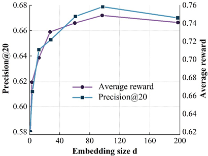
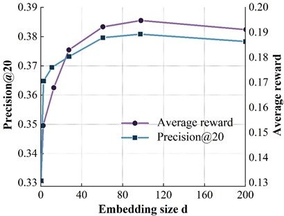
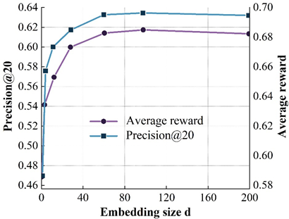
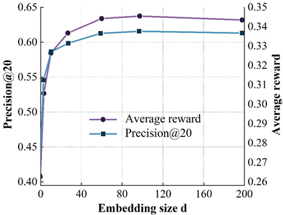
From the figure, it can be found that when the \(d\) value is small (e.g., \(d\)= 8), the model size is small and insufficient to adequately express the data features, which affects the accuracy of the model; when increasing \(d\), the accuracy of the model is then improved and reaches the peak; when continuing to increase the \(d\) value, the accuracy of the model is slightly reduced because the limited by the size of the training data, so that the model parameters are not sufficiently learned, and even if we continue to increase \(d\), the model size no longer continues to increase, thus affecting the accuracy of the model.
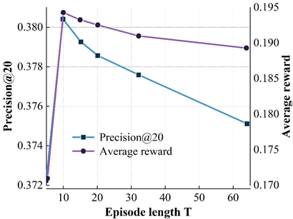
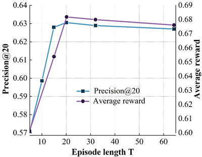
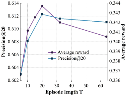
The interaction step \(T\) refers to the number of interactions between the user and the recommender system in each loop. The interaction step size is more important for reinforcement learning based recommendation algorithms.
Figure 5 shows the variation of the model’s accuracy on the four datasets for different \(T\) values. Where the X-axis represents different \(T\) values and the left and right Y-axis represent the results of the model on precision@20 and average reward metrics, respectively. From the results, it can be found that on the ML (100k) dataset, the accuracy of the DRR-att model first increases and then decreases with increasing \(T\), with the peak occurring at \(T\) = 10, and a similar situation occurs on the other three datasets. The reason for the occurrence of the above is mainly related to the balance of the exploration-utilization mechanism of the reinforcement learning recommender system during the interaction with the user. On the one hand, at the beginning of the interaction between the user and the recommender system, the recommender system needs to keep exploring to try to learn the user’s behavioral preferences. If the interaction step size is too small, it will lead to an incomplete exploration process of the recommender system, which cannot better grasp the user’s behavioral preferences, resulting in an unsatisfactory recommendation; on the other hand, with the increase of the number of interactions, the recommender system better captures the user’s behavioral preferences, and continuously utilizes this explored behavioral preferences to make a recommendation, which leads to a continuous increase of the model accuracy. When \(T\) becomes too large, excessive exploration will cause the recommender system to continuously try more “risky” recommendations, which will introduce noise to a certain extent, and will not be conducive to the exploration of the user’s interest preferences, resulting in a decline in model effectiveness.


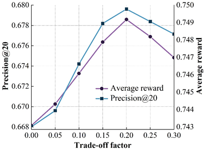
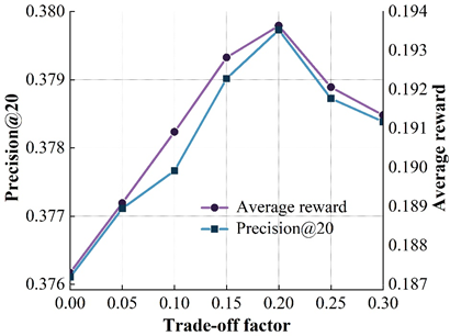
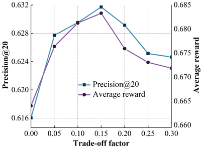
The design of the reward function is a very important factor in reinforcement learning based recommendation algorithms. Figure 6 shows the effect of different \(\alpha\) values on the model on the four datasets. Where the X-axis represents different \(alpha\) values and the left and right Y-axis represent the results of the model on the precision@20 and average reward metrics, respectively. From the variation curve of model accuracy in the figure, it can be found that the accuracy of the model on the ML (100k) dataset increases with the increase of \(\alpha\), and peaks at \(\alpha\) = 0.15. Then, the accuracy of the model starts to decrease as \(\alpha\) continues to increase. The above phenomenon occurs mainly because of the following two reasons: on the one hand, reward shaping does improve the model accuracy to a certain extent because the potential rewards are designed in order for the recommendation strategy to produce actions with better sorting performance, and thus the model sorting accuracy will be improved; on the other hand, an excessively large \(\alpha\) indicates that the potential rewards are over-weighted, and this will lead to the fact that the overall reward function will be biased towards the sorting metrics of supervised learning, which to some extent affects the exploration of user preferences by the recommender intelligence in the process of reinforcement learning, thus leading to a decrease in the accuracy of the model.
Accurate recommendation of books based on user image is to extract user characteristics on the basis of obtaining real user data, and adopt recommendation algorithms according to the analysis results to realize the recommendation service that meets the needs of readers. In this section, based on the real borrowing data of readers in a university library, the user portrait model applicable to libraries constructed by using the algorithmic model in the previous section is used to cluster library readers, construct a portrait of library readers, and analyze the results of the portrait. Based on the results of user clustering, the recommendation algorithm of collaborative filtering is used to recommend books of interest to readers, and finally the effectiveness of the recommendation results is verified through the interview method, which provides a reference for the subsequent research on accurate recommendation services in the library field.
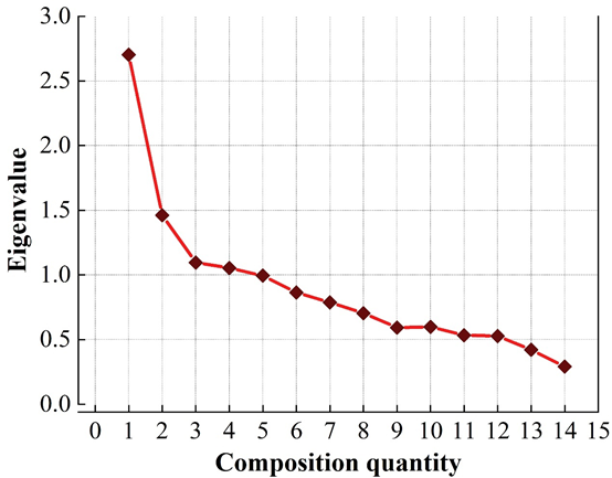
In order to extract the data that can visually represent the user characteristics from the complex data relationships, the subject variables are done dimensionality reduction with the help of SPSS software to extract the feature factors, which will be used as the classification of the labels. Initially, the extraction principle is set as the eigenvalue is greater than 1, and the number of factors is set to be obtained by maximum variance rotation method. Figure 7 shows the factor fragmentation map, Table 3 shows the variance explained rate table, and Table 4 shows the rotated component matrix. , from the results of the obtained factor fragmentation diagram, variance explanation rate table and rotated component matrix are synthesized, when 5 characteristic factors are extracted as the classification of labels, it can be seen through the variance explanation rate table that the variance explanation rate after the rotation is 53.039% of the variance of the original variable, and the results of the factor analysis are more satisfactory.
| N | Characteristic root | The difference of explanation at the forward | Differential explanation rate | ||||||
| Characteristic root | Variance interpretation rate | Cumulation | Characteristic root | Variance interpretation rate | Cumulation | Characteristic root | Variance interpretation rate | Cumulation | |
| 1 | 2.641 | 18.534 | 18.534 | 2.641 | 18.534 | 18.534 | 2.338 | 16.803 | 16.803 |
| 2 | 1.511 | 10.266 | 28.8 | 1.511 | 10.266 | 28.8 | 1.493 | 10.606 | 27.409 |
| 3 | 1.196 | 8.485 | 37.285 | 1.196 | 8.485 | 37.285 | 1.336 | 9.312 | 36.721 |
| 4 | 1.139 | 8.144 | 45.429 | 1.139 | 8.144 | 45.429 | 1.152 | 8.189 | 44.91 |
| 5 | 1.08 | 7.61 | 53.039 | 1.08 | 7.61 | 53.039 | 1.145 | 8.129 | 53.039 |
| 6 | 0.97 | 6.89 | 59.929 | ||||||
| 7 | 0.897 | 6.413 | 66.342 | ||||||
| 8 | 0.829 | 6.023 | 72.365 | ||||||
| 9 | 0.747 | 5.362 | 77.727 | ||||||
| 10 | 0.733 | 5.169 | 82.896 | ||||||
| 11 | 0.685 | 4.904 | 87.8 | ||||||
| 12 | 0.662 | 4.715 | 92.515 | ||||||
| 13 | 0.581 | 4.097 | 96.612 | ||||||
| 14 | 0.476 | 3.388 | 100 | ||||||
| Load factor | |||||
| Factor1 | Factor2 | Factor3 | Factor4 | Factor5 | |
| Operating system | 0.623 | -0.049 | 0.162 | -0.093 | 0.027 |
| programming | 0.816 | -0.082 | -0.103 | -0.029 | -0.018 |
| Computer application | 0.641 | 0.145 | 0.172 | 0.052 | 0.033 |
| Algorithmic language | 0.784 | 0.047 | 0.011 | 0.02 | -0.07 |
| automation | 0.485 | 0.141 | 0.362 | 0.159 | -0.106 |
| Engineering material | -0.03 | 0.689 | -0.074 | -0.077 | 0.127 |
| Mechanical and instrumentation industry | 0.197 | 0.609 | 0.261 | 0.188 | -0.135 |
| Metal and metal technology | -0.007 | 0.786 | -0.055 | -0.04 | -0.003 |
| Electronic communication | 0.282 | -0.131 | 0.621 | -0.099 | 0.03 |
| Electronic technology | -0.02 | 0.075 | 0.848 | 0.012 | -0.013 |
| Oil and gas industry | -0.015 | -0.015 | -0.058 | 0.723 | -0.074 |
| Water engineering | 0.011 | 0.001 | 0.02 | 0.74 | 0.145 |
| Chemical industry | -0.027 | 0.126 | -0.021 | -0.083 | 0.751 |
| Environmental science | -0.011 | -0.084 | 0.011 | 0.15 | 0.739 |
Based on the rotated component matrix, the label categorization of the library user profile is described as follows:
Label 1: “Computer” factors, which are related to the topics of operating systems, programming, computer applications, algorithmic languages and automation, and which combine to reflect readers’ needs for computer software and computer applications.
Label 2: “Mechanical” factors, which are related to engineering materials, metallurgy and metal processes and the machinery and instrumentation industry, and are closely related to the majors and research topics of the students in the Faculty of Mechanical Sciences.
Label 3: “Electronic Communications” factors, which are related to the topic of electronic communications and electronics technology.
Label 4: “Energy” factors, which are related to the oil and gas industry and water engineering, reflecting readers’ preference for books on energy topics.
Label 5: “Environmental and chemical” factors, which are related to the chemical industry and environmental sciences, synthesize the needs of the user’s college-specific role and indicate the user’s interest in environmental and chemical industry topics.
The number of user profiles depends on how well the clustering algorithm clusters all the samples, and the appropriate number of clusters is explored through the method of systematic clustering before clustering is performed using the K-means algorithm. The core of systematic clustering is that each variable is first treated as a separate class, and by calculating the distance between variables, the closer ones are merged into one class, and the more distant ones are formed into new class clusters. This is performed sequentially until all variables are categorized into appropriate classes, resulting in a significant hierarchical structure of clustering results, as shown in Figure 8.
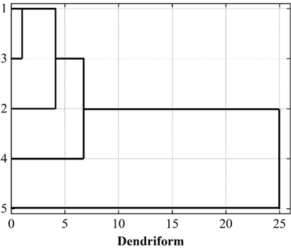
Initially, the number of clusters is selected as 3. When the number of clusters is 3, the first class contains the three feature factors of computers, electronic communications and mechanical materials, and the second and third classes represent the energy class and cyclization class, respectively, as shown in Table 5. In the case of the specified classification group k=3, K-means clustering method is used to classify the users, and the users with similar characteristics are gathered together to form different portrait groups. Also comparing the F-value and significance level of each male factor in the ANOVA table when the classification group k=4, k=5, it can be seen that when the number of clusters is 3, 4 and 5, respectively, the Sig of all five male factors are significant. When divided into 5 categories, the F-value difference of the 5 eigenfactors in Table 5 is small, and the distinction between the portraits is not obvious; when divided into 4 categories, the classification exists in a small category, so give up this option, and finally choose the number of clusters to be 3.
| Clustering number = 3 | Clustering number = 4 | Clustering number = 5 | ||||||
| F | Sig. | F | Sig. | F | Sig. | |||
| Computer class | 246.38 | 0 | Computer class | 212.454 | 0 | Computer class | 295.232 | 0 |
| Mechanical material class | 153.92 | 0 | Mechanical material class | 65.033 | 0 | Mechanical material class | 72.88 | 0 |
| Electronic communication class | 6325.759 | 0 | Electronic communication class | 155.296 | 0 | Electronic communication class | 3711.038 | 0 |
| Energy class | 8249.05 | 0 | Energy class | 5610.774 | 0 | Energy class | 4207.423 | 0 |
| cyclization | 47.034 | 0 | cyclization | 6176.923 | 0 | cyclization | 4632.686 | 0 |
When the number of clusters of user portraits is 3, the final clustering center is shown in Table 6, and each portrait is significantly different in each feature factor.
| Clustering | |||
| 1 | 2 | 3 | |
| Computer class | -1.421 | 24.372 | 0.397 |
| Mechanical material class | -2.307 | 12.974 | -3.665 |
| Electronic communication class | -3.122 | 21.225 | 1.058 |
| Energy class | 42.559 | 7.768 | 4.038 |
| cyclization | -4.511 | -5.326 | 26.391 |
Through many experiments, this paper finally determines the number of topic words N as 20, and takes the 20 topic words with larger values of word probability distribution as the characteristic topic words under different clustering groupings, and fully demonstrates the different attribute characteristics and interest preference tendencies of the group users through the distribution of the corresponding topics of the users of each group. Aggregating the above various types of labeling information as well as the proportion of demographic attributes, the final results are displayed as shown in Table 7.
| User portrait type characteristic factor | Readership 1 | Readership 2 | Readership 3 | |||
| Energy | Computer electronic communication Mechanical material | Environmental chemistry | ||||
| Classification ratio | Undergraduates | 60% | Undergraduates | 68% | Undergraduates | 65% |
| Master’s degree | 35% | Master’s degree | 30% | Master’s degree | 32% | |
| Doctoral student | 5% | Doctoral student | 2% | Doctoral student | 3% | |
| Proportion of the college | Vehicle and energy institute: | 55% | Machinery and engineering institute: | 25% | Environmental and chemical engineering institute: | 60% |
| Electrical engineering institute: | 20% | |||||
| Machinery and engineering institute: | 25% | Information science and engineering institute: | 20% | Mechanical engineering institute: | 15% | |
| Other: | 20% | Other: | 35% | Other: | 25% | |
| Group user theme interest |
Oil and gas protection oilfield gas layer
oil production development project design pipeline permeable hydrate oil gas oil gas well distribution fluid mechanical drilling storage and transportation |
Mechanical and mechanical electromechanical
automatic continuous casting material electronic technology signal machine image processing modeling programming circuit analysis control metal computer operating system wireless application communication simulation |
Chemical process pollution control green
governance environmental science triwaste catalyzed high molecular environmental protection principle water treatment air reactor chemical inspection waste treatment quality inspection |
|||
From the tag word cloud drawn in the above table to describe the portrait, we can know the attribute characteristics of the topic of interest of each reader group, so as to clearly determine the interest tendency of each reader group, summarize the characteristics of each type of portrait as follows:
The first category of users is characterized by a preference for reading books on energy topics, and most of the readers in this category usually pay attention to energy topics such as oil, natural gas, oil fields, oil and gas, storage and transportation. This group of people is mainly concentrated in the College of Vehicles and Energy, which belongs to the more specialized disciplines, and the borrowed book category is relatively single, and the reading theme is closely related to the majors and research directions studied.
The second group of users prefers resources with computer, electronic communication and mechanical themes, and the frequency of computer, communication, mechanical, simulation, modeling, control and other characteristic words is the highest, and the distribution of colleges belonging to this kind of people is mostly in the School of Mechanical Engineering, the School of Electrical Engineering and the School of Information Science and Engineering, and these colleges are characterized by the strong intersection of disciplines; with the development of the society, more and more all-around talents are needed, and the students With the development of society, there is a growing need for all-round talents, and students need to increase their knowledge and enhance their competitiveness through extensive reading. Therefore, students in the School of Mechanical Engineering are required to have basic knowledge of communications and computers, and students in the School of Information Science have dabbled in mechanical topics.
The third type of user interest tendency is the environmental and chemical theme books, the group of chemistry, environment, governance, pollution control with great enthusiasm, mainly concentrated in the more specialized College of Environmental and Chemical Engineering, focusing on the remediation of contaminated water, gas, solid, as well as potentially hazardous and toxic chemicals identification and determination, so this group of people read the theme of the chemical inspection, pollution control is closely related.
The data used includes four parts: user attribute data, book attribute data, user rating data for books and user collection borrowing data for books. The user attribute data includes the user’s age, gender, and specialty, etc. Some of the user attribute data are shown here, as shown in Table 8.
| User ID | Gender | Age | Professional ID |
| 20201314031 | 1 | 19 | 80622 |
| 20201314032 | 1 | 19 | 50107 |
| 20201314033 | 0 | 21 | 91150 |
| 20201314034 | 1 | 20 | 23508 |
| 20201314035 | 0 | 18 | 71010 |
| 20201314036 | 1 | 20 | 41310 |
| 20201314037 | 1 | 19 | 31512 |
| 20201314038 | 0 | 23 | 31008 |
| 20201314039 | 0 | 21 | 40301 |
| 20201314040 | 1 | 20 | 50210 |
Book attribute features consist of 10 book attributes, book attributes include: programming, algorithmic language, metal craft, electronic communication, oil and gas industry, machinery, water engineering, environmental science, chemistry, energy. When a book has a certain feature, the corresponding value of the attribute is 1, and vice versa is 0. Some of the book attribute data are shown in Table 9.
| Book ID | Attribute 1 | Attribute 2 | Attribute 3 | Attribute 4 | Attribute 5 | Attribute 6 | Attribute 7 | Attribute 8 | Attribute 9 | Attribute 10 |
| 43 | 0 | 0 | 1 | 0 | 1 | 1 | 0 | 1 | 0 | 0 |
| 44 | 0 | 1 | 0 | 0 | 1 | 1 | 1 | 0 | 1 | 0 |
| 45 | 1 | 1 | 1 | 1 | 0 | 0 | 1 | 1 | 1 | 1 |
| 46 | 1 | 1 | 0 | 1 | 1 | 0 | 1 | 1 | 0 | 1 |
| 47 | 1 | 0 | 0 | 1 | 1 | 0 | 1 | 1 | 1 | 0 |
| 48 | 1 | 0 | 1 | 1 | 1 | 1 | 0 | 0 | 0 | 0 |
| 49 | 0 | 1 | 0 | 0 | 0 | 1 | 1 | 1 | 1 | 1 |
| 50 | 1 | 1 | 1 | 0 | 0 | 0 | 1 | 0 | 0 | 1 |
| 51 | 0 | 0 | 1 | 0 | 0 | 1 | 0 | 1 | 0 | 0 |
| 52 | 1 | 1 | 0 | 1 | 1 | 0 | 1 | 1 | 1 | 0 |
Some of the data on user ratings of books are shown in Table 10.
| User ID | Book ID | Scoring |
| 20211109097 | 34 | 5 |
| 20191417158 | 28 | 1 |
| 20191725219 | 63 | 3 |
| 20202033280 | 75 | 4 |
| 20202341341 | 18 | 3 |
| 20212649402 | 44 | 3 |
| 20202957463 | 93 | 4 |
| 20203265524 | 86 | 3 |
| 20193573585 | 73 | 4 |
The user performs collection and lending operations on the book, and it is 1 if it performs collection or lending operations, and 0 if it performs the opposite. Some of the user behavior data is shown in Table 11.
| User ID | Book ID | Collect | Borrowing |
| 20212649402 | 27 | 0 | 1 |
| 20203265524 | 39 | 0 | 0 |
| 20211725219 | 54 | 0 | 1 |
| 20190828666 | 73 | 1 | 0 |
| 20190366575 | 21 | 1 | 0 |
| 20201566323 | 85 | 0 | 1 |
| 20211366072 | 63 | 1 | 0 |
| 20210965821 | 80 | 0 | 1 |
| 20201255697 | 95 | 1 | 1 |
Applying the corresponding data to the model in this paper, some of the recommendation results produced are shown in Table 12. Recommendations are generated for all the selected users, and the recommendation results are more diverse, which fully demonstrates that the recommendation model proposed in this paper can effectively solve the problem of not being able to recommend due to data sparsity and the problem of low recommendation coverage. It can be seen that the recommendation model proposed in this paper has obvious improvement compared with the traditional recommendation algorithm.
| User ID | Book ID | |||||
| 20213431456 | 35 | 73 | 51 | 1 | 37 | 8 |
| 20216966675 | 97 | 41 | 71 | 31 | 76 | 18 |
| 20200501893 | 92 | 79 | 8 | 73 | 48 | 70 |
| 20224037111 | 58 | 40 | 14 | 67 | 57 | 13 |
| 20207572330 | 52 | 78 | 12 | 33 | 27 | 40 |
| 20231107548 | 41 | 85 | 81 | 12 | 23 | 29 |
| 20194642766 | 43 | 53 | 84 | 42 | 62 | 39 |
| 20208177985 | 65 | 21 | 51 | 72 | 26 | 49 |
In this paper, we propose a personalized preference acquisition algorithm based on user profiles to achieve personalized information recommendation for intelligent libraries. After extracting user attribute features and behavioral features, we train to obtain a behavioral model that can predict the user’s preferences, and generate a preference recommendation list. After experiments on the dataset and put into practical applications, it is found that the model in this paper outperforms the rest of the models on the experimental dataset in all observation items. The designed state representation module improves the accuracy of modeling user states and thus improves the ranking performance of the model. The personalized recommendation results provided by the state representation module based on reinforcement learning are better compared to the baseline model. In practical applications, after determining the number of clusters in the user profile as 3, all the selected users have diverse recommendations, and it can be considered that the recommendation model proposed in this paper has obvious improvement compared with the traditional recommendation algorithm.