
The study of reduced words of permutations in connection with tableaux dated back to the work [9] of Alain Lascoux and Mercel-Paul Schützenberger in which they partitioned the set of reduced words of a given permutation into niplatic classes and characterised every element of each of the classes by its \(Q\)-symbol. This is closely related to the RSK-correspondence. There have been a significant amount of work along this direction ever since, the reader is referred to [3,6,8,11,12,13,14] for further reading.
In this paper, we study the reduced word graphs of the permutations \(_{n}w\) of the form \[, \ {\rm for} \ \ n\geq 4. \tag{1}\]
These permutations are characterised by the hook cycle type \((n-2, 1,1)\) with consecutive fixed points at the positions \(n-1\) and \(n-2\). The characterisation realises a bijection between the set of reduced words of \(_{n}w\) and a certain sub-collection of the set of row-strict tableaux \(\tau\) shaped \((n-2,1,1)\). The entries of each tableau encode the positions of ascents and descents of every reduced words of \(_{n}w\) with respect to a specific row-reading. This gives rise to a closed formula for counting the number of reduced words of \(_{n}w\) in terms of multinomial coefficients. It turns out that there is an isomorphism between the graph of reduced words of each of the permutations \(_{n}w\) and the Hasse diagram \(\mathcal{R}^{_{\tau}w}_{n}\) of the sub-collection of row-strict tableaux \(\tau\). It is also observed that the set of row-readings of the sub-collection of row-strict tableaux \(\tau\) is precisely the set of Grassmannian permutations with a unique descent at \((n-2)\). In fact, these are exactly all the Grassmannian permutations whose associated partition fits into the rectangle \(\square_{n-2\times 2}\). It is well-known that the usual q-binomial coefficient q-counts the number of such partitions: \[\label{eq2} \left[ n \choose n-2\right]_q =\sum_{\lambda} q^{|\lambda|}, \tag{2}\] where \(|\lambda|\) denotes the number partitioned by \(\lambda\). This has an interesting implication in algebraic geometry in that these partitions index the Schubert varieties of the Grassmannian \({\rm Gr}(2,n)\), the variety of 2-planes in an \(n\)-dimensional complex vector space. The Poincaré polynomial of the integral cohomology ring \(H^{\ast}({\rm Gr}(2,n),{\mathbb{Z}})\) of the Grassmanian \({\rm Gr}(2,n)\) is the \(q\)-binomial coefficient given in (2) and Schubert cycles are cohomology classes that are Poincaré dual to the fundamental homology cycles of Schubert varieties in the Grassmannian. The observation reveals a fundamental connection between the graph \(\mathcal{G}_{_{n}w}\) of the reduced words of the permutation \(_{n}w\) and the graph \(\mathcal{G}_{(n-2)\Delta_{2}\cap {\mathbb{Z}}^{2}}\) of \((n-2)\)-fold dilation of the standard 2-simplex. That is, to every lattice point a in \((n-2)\Delta_{2}\cap {\mathbb{Z}}^{2}\) there is a fitted partition \(\lambda\) and a weight \({\bf m}_{\bf a}\) such that the length of the Grassmannian permutation \(w(\lambda)\) is \({\bf m}_{\bf a}\).
This paper is orgainized as follows. Some necessary backgrounds on the symmetric group \(\frak{S}_{n}\) are reviewed and two preliminary results are given in Section 2. The bijecton between the vertex set of the graph \(\mathcal{G}_{_{n}w}\) of reduced words of the permutation \(_{n}w\) and the sub-collection of row-strict tableaux \(\tau\) of shape \((n-2,1,1)\) which brings out the closed formula for the order of the graph is established in Section 3. The symmetry in the structure of the graph \(\mathcal{G}_{_{n}w}\) is exploited in the same section to give the vertex-degree polynomials \({\rm P}_{\mathcal{G}_{_{n}w}}(d)\) for \(n\geq 4\) and their generating series. In Section 4 we give a poset of the sub-collection of row-strict tableaux \(\tau\) and establish an isomorphism between the graph \(\mathcal{G}_{_{n}w}\) and the Hasse diagram of the row-strict tableaux. We show that the Hasse diagram is graded by identifying it with the sub-poset of Grassmannian permutations induced by the strong Bruhat graph of the symmetric group \(\mathfrak{S}_{n}\). In section 5 we give a construction of poset of the lattice points \({(n-2)\Delta_{2}\cap {\mathbb{Z}}^{2}}\) of \((n-2)\)-fold dilation of the standard \(2\)-simplex using lexicographic ordering. The Hasse diagram of the poset is graded such that the rank polynomial is a refinement of the Ehrhart polynomial of the simplex. The graph of lattice points is realised as the Hasse diagram of the poset.
It is well-known that the symmetric group \(\mathfrak{S}_{n}\) on the set \([n]:=\{1,\ldots, n\}\) is finitely presented. That is,
\[\mathfrak{S}_{n}= \langle s_1,\dots, s_{n-1} : s_{i}^{2} =e,\ s_{i}s_{j} = s_{j}s_{i} , \ s_{i}s_{i+1}s_{i} = s_{i+1}s_{i}s_{i+1} \rangle.\]
The generators \(s_1, s_2,\dots, s_{n-1}\) are simple transpositions, each of which is an involution. The relations \(s_{i}s_{j} = s_{j}s_{i}\) for \(\mid i-j\mid > 1\) and \(s_{i}s_{i+1}s_{i} = s_{i+1}s_{i}s_{i+1}\) for \(1\leq i\leq n-2\) are called commutation and braid relation respectively. We shall adopt one-line notation for the elements in \(\mathfrak{S}_{n}\). The length \(\ell(w)\) of the permutation \(w\in\mathfrak{S}_{n}\) is given by the number of inversions in \(w\),
\[\ell(w) = |\{(i,j)\in [n]^{2} : w(i)> w(j), 1\leq i<j\leq n\}|,\] and the length generating function of the symmetric group \(\mathfrak{S}_{n}\) is given by \[\label{eq2.1} G_{\mathfrak{S}_{n}} (q)= \prod^{n}_{k=1} \frac{q^{k}-1}{q-1}. \tag{3}\]
The symmetric group \(\mathfrak{S}_{n}\) is a poset under the Bruhat order, that is, for \(v, v'\in \mathfrak{S}_{n}\), \(v < v'\) if \(v'\) is realised from \(v\) by interchanging \(v_{i}\) and \(v_{j}\) where \(i<j\) and \(v_{j} = v_{i}+1\). This defines the strong Bruhat order on \(\mathfrak{S}_{n}\). It is important to note that the strong Bruhat order encodes some geometric interpretations as it describes the inclusion ordering of Schubert varieties of certain homogeneous spaces such as flag manifolds and Grassmannians [4,5]. The poset of \(\mathfrak{S}_{n}\) with respect to the Bruhat order is graded and the length generating function described in Eq. (3) is its rank function [4].
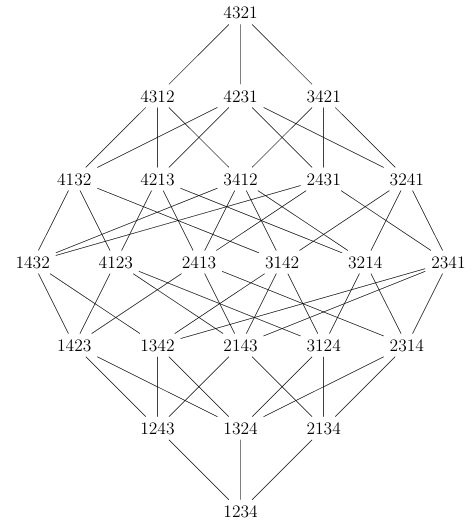
Example 2.1. The Hasse diagram of \(\mathfrak{S}_{4}\) with respect to the strong Bruhat order is given in ’Figure1 and its rank function is \(\displaystyle G_{\mathfrak{S}_{4}} (q)= q^6+ 3q^5 + 5q^4 + 6q^3+ 5q^2 + 3q + 1 .\)
Recall that the length of \(w\in\frak{S}_{n}\) is invariant under inversion \(w\mapsto w^{-1}\) and conjugation \(w\mapsto w_{0}ww_{0}\), where \(w_{0}= [n,n-1,n-2,\dots, 3,2,1]\). Therefore, \(\ell(w)=\ell(w^{-1})=\ell(w_{0}ww_{0})=\ell(w_{0}w^{-1}w_{0})\). The descent set Des(\(w\)) of \(w\) is given by Des(\(w\))=\(\{i : w_{i}> w_{i+1}\}\). If the product \(s_{a_{1}}s_{a_{2}}\cdots s_{a_{p}} = w\) is such that \(p=\ell(w)\) then the sequence \({\bf a} = a_{1}a_{2}\cdots a_{p}\) is called a reduced word for \(w\). The descent set Des(a) of the reduced word a=\(a_{1}a_{2}\cdots a_p\) is given by Des(a)=\(\{j : a_{j}> a_{j+1}\}\), likewise the ascent set Asc(a) of a is given by Asc(a)=\(\{j : a_{j} < a_{j+1}\}\). The reduced word of \(w\) is not unique in that another reduced word of \(w\) can be realised by applying a series of braid and commutation relations. This observation gives rise to the graph \(\mathcal{G}_{w}\) of reduced words of the permutation \(w\) in which the reduced words of \(w\) constitute the vertices of the graph and edges are given by any pair of reduced words where one is obtained from the other by a braid or commutation relation. We denote the set of reduced words for \(w\in \frak{S}_{n}\) by \(R(w)\) and its cardinality by \(r(w)\).
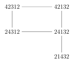
Example 2.2. If \(w = 35124\) then \(R(w)=\{42312, 24312, 42132, 24132,21432 \} \ \ {\rm and} \ \ r(w)=5.\) The graph \(\mathcal{G}_{35124}\) of the reduced words of the permutation \(w=35124\) is given by \("{\rm Figure \ 2 }"\).
If \(w=[6,5,4,2,3,1]\) then \(r(w) =64,064\). A natural question is the following: Given any permutation \(w\in\mathfrak{S}_{n}\), how do we compute \(r(w)\)? The question is interesting due to fact that \(r(w)\) encodes a number of combinatorial and geometric interpretations for certain class of permutations. In order to compute \(r(w)\), Stanley [12] introduced a certain function \(F_{w}\) called Stanley symmetric function. It turns out that the coefficient of the square free monomial in \(F_{w}\) is number of the reduced words of \(w\). This is given by \[\label{eq2.2} r(w) = \sum_{\lambda\vdash \ell(w)} a_{\lambda(w)} f^{\lambda}. \tag{4}\]
It follows from the fact that \(F_{w}\), being a symmetric function, can be expanded uniquely as an integral linear combination of the Schur functions, that is, \(\displaystyle F_{w} = \sum_{\lambda\vdash \ell(w)}a_{\lambda(w)} s_{\lambda}, \ a_{\lambda(w)}\in{\mathbb{Z}}\). The coefficient of the square free monomial in \(s_{\lambda}\) is the hook length \(f^{\lambda}\).The reader is referred to [12] for further detail. Unfortunately, there is no general closed formula for the computation of \(r(w)\) for any given \(w\in\mathfrak{S}_{n}\). However, for \(w_{0}\), the longest permutation in \(\mathfrak{S}_{n}\), Stanley [12] gave a closed formula for \(r(w_{0})\) as \[\label{eq2.3} r(w_{0})= \frac{{n\choose 2}!}{1^{n-1}3^{n-2}5^{n-3}\cdots (2n-3)^{1}}. \tag{5}\]
This is precisely the number \(f^{n-1,n-2,\dots, 3,2,1}\) of standard tableaux of shape \(\lambda =(n-1,n-2,\dots, 3,2,1)\). The goal of this paper is to study the graphs of reduced words of the permutations \(_{n}w\) in the family \(\mathcal{W}\subset\cup_{n\geq 4}\mathfrak{S}_{4}\). These permutations are of the form: \[\label{eq2.4} _{n}w = [n,1,2,3,\dots, n-4, n-2, n-1, n-3], \ {\rm for} \ \ n\geq 4. \tag{6}\] For instance, \(_{4}w = 4231, \ _{5}w = 51342, \ _{6}w = 612453\), etc. We look at the graphs of reduced words of these permutations due to their interesting symmetry and deep connection with the Schubert varieties of Grassmannian Gr\((2,n)\), of 2-dimensional subspaces in an \(n\)-dimensional vector space over the complex field.
Proposition 2.3. Let \(w\in\mathfrak{S}_{n}\) such that \(w\) is of the form \[[n,1,2,3,\dots, n-4, n-2, n-1, n-3], \ {\rm for} \ \ n\geq 4.\] Then the following properties hold
(i) \(w\) has length \(n+1\).
(ii) \(w\) is of the cycle type \((n-2,1,1).\)
(iii) The consecutive fixed points of \(w\) occur at the positions \(n-2\) and \(n-1.\)
(iv) There are only two descents in \(w\).
Proof. Recall that the length of a permutation is given by the number of inversions in the permutation.
(i) Looking at the form of \(w\), there are exactly \(n-1\) inversions associated with the value \(n\) since every value to the right of \(n\) is strictly less that \(n\). Also each of the value \(n-2\) and \(n-1\) has exactly one inversion associated to it. The values \(1,2,3,\dots,n-4\) are in increasing order so there is no inversion. Therefore, \(w\) has \(n+1\) inversions.
(ii) The partition of the set \([n]:=\{1,2,\dots,n\}\) via \(w\) realises the orbit \(\{1, w(1), w^{2}(1), \ldots \\ ,w^{n-3}(1)\}\) of \(1\) as the only orbit of \([n]\) which has more than one element. So \(w\) is an \((n-2)\)-cycle.
(iii) From (ii), the orbits of \(n-2\) and \(n-1\) are respectively, \(\{n-2\}\) and \(\{n-1\}\).
(iv) The formulation of \(w\) ensures the descents only occur at the first and last but one position. ◻
Proposition 2.4. Let \(w,\sigma\in\mathfrak{S}_{n}\) such that \(w\) is of the form \[[n,1,2,3,\dots, n-4, n-2, n-1, n-3], \ {\rm for} \ \ n\geq 4,\] and \(\sigma\) is the reverse of \(w\). Then \(\ell(w)+\ell(\sigma) = {n\choose 2}\).
Proof. By definition, \(\sigma_{i} = w_{n+1-i}\) for \(1\leq i\leq n\), so the permutation \(\sigma\) is of the form \([n-3,n-1,n-2,n-4,\dots, 3,2,1,n]\). The value \(n-3\) has \(n-4\) inversions associated to it, the value \(n-1\) has \(n-3\) associated inversions while the value \(n-2\) gives \(n-4\) inversions. There are \({n-4\choose 2}\) inversions within the values \(n-4,\dots,3,2,1\) being in decreasing order. Therefore, \(\ell(\sigma)=\frac{n^{2}-3n-2}{2}\). Recall that \(\ell(w)=n+1\) so that \(\ell(w)+\ell(\sigma) = {n\choose 2}\). ◻
In this section we study the graphs of reduced words of the permutations \(_{n}w\) for \(n\geq 4\). The reduced words constitute the vertices of the graphs in question while the edges are given either by commutation or braid relation.
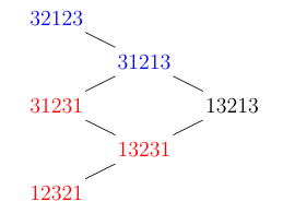
Example 3.1. For \(n = 4\), then the set \(R(_{4}w)\) of reduced words of the permutation \(_{4}w = 4231\) is given by
\[\label{eq3.1} R(_{4}w) =\{ {\color{blue}32123, 31213, } 13213, {\color{red}{31231, 13231, 12321}} \}. \tag{7}\] Its graph, denoted by \(\mathcal{G}_{_{4}w}\) is illustrated in Figure 3 .
The first goal here is to give a closed formula for the order of the graph \(\mathcal{G}_{_{n}w}\) for any \(n\), that is, the number of the vertices of \(\mathcal{G}_{_{n}w}\). This is the cardinality \(r(_{n}w)\) for the set \(R(_{n}w)\). The closed formula will be realised via a bijection of \(R(_{n}w)\) with a certain combinatorial object, therefore, the following proposition is very important in order to count the number of vertices of the graph \(\mathcal{G}_{_{n}w}\).
Proposition 3.2. Let \({\bf a}\in R(_{n}w)\) then a has exactly 2 ascents and \(n-2\) descents.
Proof. Notice that by induction there only two degree one vertices in the graph \(\mathcal{G}_{_{n}w}\) of the reduced words of the permutation \(_{n}w\) with 2 ascents each, these are \((n-1)(n-2)(n-3)\cdots 321(n-2)(n-1)\) and \((n-3)(n-2)(n-1)(n-2)\cdots 321\). Since these vertices are respectively located at the top and bottom of the graph, every reduced word of \(_{n}w\) lies on the paths between them. The result follows then by noticing that the number of ascents or descents is invariant under commutation and braid relations. ◻
We now introduce the combinatorial object \(\mathcal{C}_{n-2,1,1},\) called the recorder, which shall simultaneously keep track of both descent and ascent positions of every reduced word of the permutation \(_{n}w\). We recall some basic facts about partitions. The reader is referred to [6,10,13] for further details on integer partition theory. A partition \(\lambda\) of \(n\in{\mathbb{N}}\) denoted \(\lambda\vdash n\) is a list \(\lambda=(\lambda_1\geq\lambda_2\geq\cdots\geq\lambda_k)\) such that \(\lambda_1+\lambda_2+\dots +\lambda_k= |\lambda|=n\). To each partition \(\lambda\vdash n\) there is an associated diagram \(Y(\lambda)\) called the Young diagram of shape \(\lambda\) consisting of \(|\lambda|\) boxes having \(k\) left justified rows with row \(i\) containing \(\lambda_i\) boxes for \(1\leq i\leq k\).
Example 3.3. If \(\lambda = (5,4,3,2,1)\) then its Young
diagram is given by
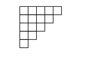
There are many ways of describing a Young tableau associated with the Young diagram of shape \(\lambda\vdash n\). We care about the row-strict tableaux which are given by the filling the boxes of the Young diagram of shape \(\lambda\vdash n\) with numbers from the set \([n]:=\{1,\dots,n\}\) such that the numbers in the rows strictly increase from left to right. Let \({\rm RST}_{n}(\lambda)\) denote the set of all row-strict tableaux of shape \(\lambda=(\lambda_{1},\lambda_{2},\dots,\lambda_{k})\vdash n\). The cardinality \(|{\rm RST}_{n}(\lambda)|\) of the set given by the multinomial coefficient: \[\label{eq3.2} |{\rm RST}_{n}(\lambda)|={n\choose{\lambda_{1},\dots,\lambda_{k}}}. \tag{8}\]
The focus is on the sub-collection of row-strict tableaux of the hook shape \((n-2,1,1)\vdash n\), where \(n\geq 4\).
Defnition 3.4. A row-strict tableau \(\tau\in {\rm RST}_{n}(n-2, 1,1)\) is said to be a recording row-strict tableau if the numbers in the last two boxes of the first column strictly decrease downward.
Example 3.5.

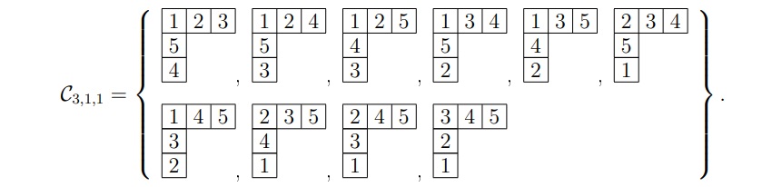
Proposition 3.6. Let \(\displaystyle \mathcal{C}_{n-2, 1,1}\) be the set of recording row-strict tableaux in \(\displaystyle {\rm RST}_{n}(n-2, 1,1)\). Then \(\displaystyle |\mathcal{C}_{n-2, 1,1}|= \frac{1}{2} {n\choose{n-2, \ 1,\ 1}}\).
Proof. The row-strict filling of the shape \((n-2,1,1)\vdash n\) requires \(\displaystyle {{n}\choose n-2}\) choices for the first row, \(\displaystyle {{2}\choose 1}\) for the second row and \(\displaystyle{1\choose 1}\) for the last row. Therefore, \(\displaystyle |\mathcal{C}_{n-2, 1,1}|={\frac{1}{2}}{n\choose n-2}\cdot {2\choose 1}\cdot {1\choose 1 }\), since \(\displaystyle \mathcal{C}_{n-2, 1,1}\), by definition, requires numbers in the last two boxes of the first column to strictly decrease downward. ◻
Example 3.7. There are 20 row-strict tableaux associated to the Young diagram of the shape \(\lambda=(3,1,1)\), that is,
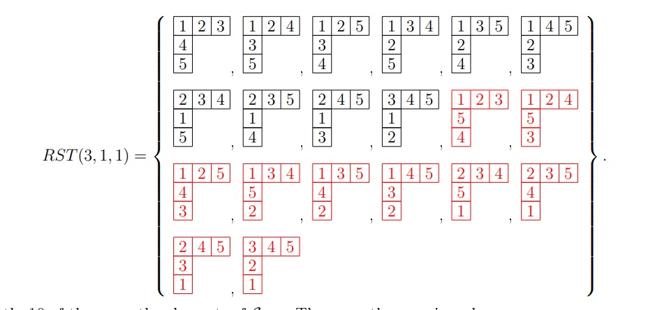 Exactly 10 of them are the elements of \(\mathcal{C}_{3, 1,1}.\) These are the ones
in red.
Exactly 10 of them are the elements of \(\mathcal{C}_{3, 1,1}.\) These are the ones
in red.
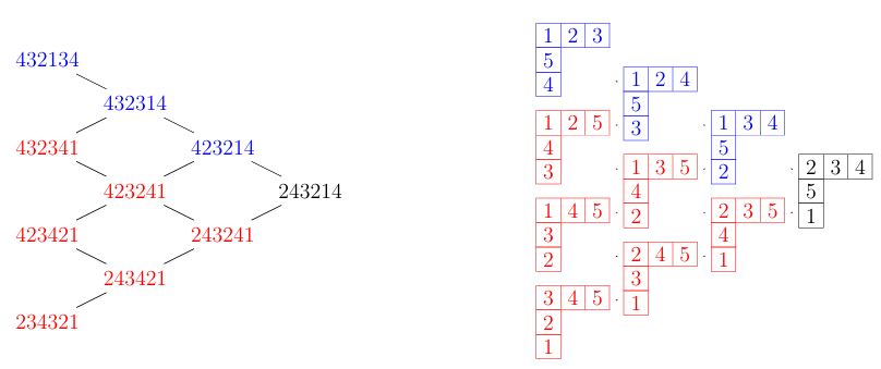
We now establish a bijection between the set \(R(_{n}w)\) of reduced words of the permutation \(_{n}w\) and the set \(\mathcal{C}_{n-2, 1,1}\) of recording row-strict tableaux in \({\rm RST}_{n}(n-2, 1,1),\) as illustrated in Figure 4. It is important to first discuss the classification of the reduced words in \(R(_{n}w)\).
Theorem 3.8. The permutation \(_{n}w\) only admits reduced words of the following types:
(I) word starting with \(n-3\) and ending with \(n-1\);
(II) words starting with \(n-1\) and ending with \(n-1\);
(III) words ending with \(1\);
The number of the reduced words of the three types is \(1\), \(n-2\) and \(\displaystyle{n-1 \choose 2}\), respectively.
Proof. We will prove the statement inductively on \(n\). In the case \(n=4\), since the length \(\ell(_{4}w) = 5\), the six reduced words of \(_{4}w\) are of length \(5\) and all these statements are straightforward; see Figure 3. For the induction step, all \(\displaystyle{n-1\choose 2}\) reduced words of length \(n\) for \(_{n-1}w, \ n\geq 4\) can be upgraded to \(\displaystyle{n\choose 2}\) reduced words of length \(n+1\) for \(_{n}w\) by increasing the length of each reduced word by one and sticking to the pattern. This is done by identifying the special reduced word from each type, the starting reduced word for each type. The special reduced word of type(II) for \(_{n-1}w\) is \((n-2)(n-3)\cdots321(n-3)(n-2)\). Following the pattern, it is upgraded to \((n-1)(n-2)\cdots321(n-2)(n-1)\), the special reduced word of type(II) for \(_{n}w\). There are exactly \(n-3\) relations starting with the special word to realise the remaining members of the type. This accounts for the \(n-2\) membership for type(II). Next, the special reduced word of type(I) for \(_{n-1}w\) is \((n-4)(n-2)(n-3)\cdots321(n-2)\). Using the same pattern, it is promoted to \((n-3)(n-1)(n-2)\cdots321(n-1)\),the special reduced word of type(I) for \(_{n}w\). There is no relation starting from this special word to realise other members of the type. Hence, it is the only one in its type. Lastly, the special reduced word of type(III) for \(_{n-1}w\) is \((n-4)(n-3)(n-2)(n-3)\cdots 321\). This is also uplifted to \((n-3)(n-2)(n-1)(n-2)\cdots 321\), the special word of type(III) for \(_{n}w\). Moving upward from this reduced word, there are \((n-2)(n-1)\) relations to realise all the \(\displaystyle{n-1 \choose 2}\) members within the type. ◻
Considering the structure of the graph \(\mathcal{G}_{_{n}w}\) of the permutation \(_{n}w\) in Figure 4, words of type (III) form a triangle in which edges are red, those of type (II) form a further parallel side of blue edges and the unique word of type (I) is the apex through which we have the line of symmetry. These give rise to the type-polynomial \({\rm P}_{n-2, 1,1}(t)\) of the set \(R(_{n}w)\) which keeps track of the size of each sub-division; \[\label{eq3.3} {\rm P}_{n-2, 1,1}(t)=\sum _{i=1}^{3} {n-4+i \choose n-3} t^{i}. \tag{9}\]
For example, The type-polynomial for the permutation \(_{5}w\) is \(\displaystyle {\rm P}_{3, 1,1}(t) = t +3t^2+6t^3\), that is, \(R(_{5}w)\), the number of reduced of the type (I), type (II) and type (III) in \(R(_{5}w)\) is 1, 3 and 6, respectively .
Remark 3.9. The type-polynomial \({\rm P}_{n-2, 1,1}(t)\) of the graph \(\mathcal{G}_{_{n}w}\) is closely connected with the Ehrhart polynomial of the \((n-2)\) dilation of the standard 2-simplex \(\Delta_{2}\) in that both of than count the number of reduced words and lattice points respectively which coincide. The reader is referred to [10] for more details on Ehrhart polynomials.
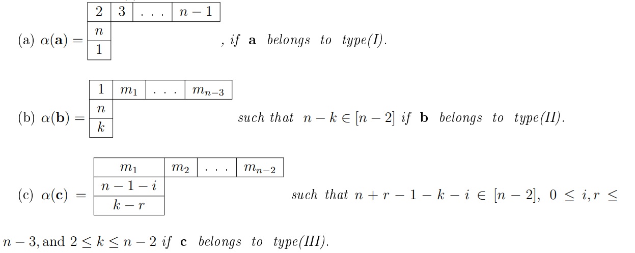
Theorem 3.10. There is a bijection \(\alpha\) between the set \(R(_{n}w)\) of reduced words of the permutation \(_{n}w\) and the set \(\mathcal{C}_{n-2, 1,1}\) of recording row-strict tableaux satisfying the following:
Proof. First notice from Proposition 3.6 and Theorem 3.8 that the two sets \(R(_{n}w)\) and \(\mathcal{C}_{n-2, 1,1}\) share the same cardinality.
(a) Since \({\bf a}\in R(_{n}w)\) is
of type(I), it is the only one of the type and has the form \((n-3)(n-1)(n-2)\cdots321(n-1)\) of length
\(n+1\). The two ascents are in the
positions \(1\) and \(n\), therefore 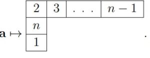
(b) Since \({\bf b}\in R(_{n}w)\) is
of type(II), there are \(n-2\) of such
reduced words. The special one is of the form \((n-1)(n-2)\cdots321(n-2)(n-1)\). The two
ascents are located in the \(n^{th}\)
and \((n-1)^{th}\) positions.
Therefore, 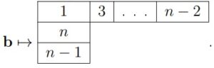 . The indicators
\(n-k\in[n-2]\) can be used to realise
the remaining \(n-3\) maps within the
type.
. The indicators
\(n-k\in[n-2]\) can be used to realise
the remaining \(n-3\) maps within the
type.
(c) Since \({\bf c}\in R(_{n}w)\) is
of type(III), there are \(n-1\choose
2\) reduced words in the type. The special one is of the form
\((n-3)(n-2)(n-1)(n-2)\cdots 321\).
This is at the lower end of the graph.Thus, the two ascents are at the
first and second positions. Therefore,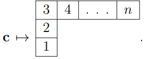 . This occurs
when \(i=n-3, k=2, r=1\). The remaining
\(\frac{n^2-3n}{2}\) maps are obtained
by applying the conditions \(n+r-1-k-i\in[n-2], \ 0\leq i,r\leq n-3, {\rm and}\
2\leq k\leq n-2\). ◻
. This occurs
when \(i=n-3, k=2, r=1\). The remaining
\(\frac{n^2-3n}{2}\) maps are obtained
by applying the conditions \(n+r-1-k-i\in[n-2], \ 0\leq i,r\leq n-3, {\rm and}\
2\leq k\leq n-2\). ◻
Theorem 3.11. Let \(\mathcal{G}_{_{n}w}\) be the graph of reduced words of the permutation \(_{n}w\). Then the order \(r(_{n} w)\) of \(\mathcal{G}_{_{n}w}\) is given by the half of the multinomial coefficient; \[r(_{n}w) = \frac{1}{2} {n\choose{n-2, \ 1,\ 1}}.\]
Proof. It follows from the bijection between the set \(R(_{n} w)\) of the reduced words of the permutation \(_{n}w\) and the set \(\mathcal{C}_{n-2, 1,1}\) of recording row-strict tableaux described in Theorem 3.8. The reduced words of \(R(_{n}w)\) have precisely \(n-2\) descents and 2 ascents each by Proposition 2.3. Thus, for each \({\bf a}\in R(_{n}w)\) there is a unique recording row strict tableau \(\tau\in\mathcal{C}_{n-2, 1,1}\) such that the entries in the first row record the positions of descents in a while the last two rows capture the location of ascents in the same reduced words. ◻
Remark 3.12. The bijection interprets \(r(_{n}w)\) as the number of certain sub-collection of row-strict tableaux of shape \((n-2,1,1)\) following the interpretation [12] of \(r(w_0)\) as the number of standard Young tableaux of shape \((n-1,n-2,\dots, 3,2,1)\). Whereas, Theorem 3.8 realises \(r(_{n}w)\) as a triangular number \(\displaystyle {n\choose 2},\) being the sum of the cardinalities of the three sub-divisions of the set \(R(_{n}w)\). It turns out that triangular numbers are connected with many combinatorial objects. We shall explore how some of these objects interact with the graph \(\mathcal{G}_{_{n}w}\) in the subsequent sections. It is also important to note that the triangular number can also be realised with reference to the lengths of the permutation \(_{n}w\) and its reverse \(\sigma\), as shown in Proposition 2.4.
Example 3.13. Given \(_{5}w=51342\), its reverse \(\sigma=24315\), so \(\ell(51342)+\ell(24315)={5\choose 2}\). There are precisely 10 reduced words for the permutation \(_{5}w\).
We shall describe in the next section a poset \((\mathcal{C}_{n-2, 1,1}, \leq)\) of recording row-strict tableaux whose Hasse diagram preserves the structure of the corresponding graph of reduced words.
The degree of a vertex in \(\mathcal{G}_{_{n}w}\) is determined by the number of all possible moves (braid and commutation) present in the reduced word. For instance, the vertex \(423241\) in \(\mathcal{G}_{_{5}w}\) is of degree 4 since it has 3 commutations and one braid.The symmetry of the graph \(\mathcal{G}_{_{n}w}\) with respect to the orientation displayed in Figure 5 gives a convenient way of keeping track of the degree of every vertex. Notice that the graph is symmetric along the horizontal line through the apex, the special reduced word of type I. A vertex \(v\) of the graph \(\mathcal{G}_{_{n}w}\) of the reduced words of \(_{n}w\) is said to be inner if it is of degree 4.
Lemma 3.14. Let \(v\) be a vertex of the graph \(\mathcal{G}_{_{n}w}\) of the reduced words of \(_{n}w\). Then the degree of \(v\) is at most \(4\).
Proof. It suffices to give the analysis of the degree of outer and inner vertices in the structure of \(\mathcal{G}_{_{n}w}\) with respect to Figure 5. Since the vertex set \(R(_{n}w)\) of the graph \(\mathcal{G}_{_{n}w}\) can be divided into three types, The special word of type (I) has degree 2 being the apex, the end vertex through which the only line of symmetry exists for the graph. The special word of type(II) has degree one being at the extreme of the NE-edges and all other vertices between the special words of types (I) and (II) along NE-edges have degree 3. Similarly, the special word of type(III) has degree one being at the extreme of the SE-edges and all other vertices between the special words of types (I) and (III) along SE-edges have degree 3. All the vertical disconnected vertices that lie between the special words of types (II) and (III) have degree two. All these constitute the outer vertices of the graph. The remaining \(n-3\choose 2\) vertices, \(n\geq 5\) are the inner vertices of the graph. They are precisely degree 4, that is, there are exactly 4 relations in each of them. One of such is of the form \((n-1)(n-3)(n-2)(n-3)\cdots32(n-1)1\) from which others can be gleaned. ◻
Remark 3.15. The degree bound is very sharp. In fact, every graph in the family \(\mathcal{W}\) except \(\mathcal{G}_{_{4}w}\) attains the bound. We now give the distribution of degrees of the vertices of \(\mathcal{G}_{_{n}w}\) in what follows.
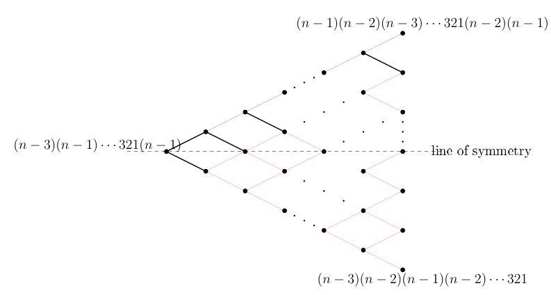
Theorem 3.16. Let \(\mathcal{G}_{_{n}w}\) be the graph of reduced words of the permutation \(_{n}w\). Then the vertex-degree polynomial is given by \[{\rm P}_{\mathcal{G}_{_{n}w}}(d)= 2d +(n-2)d^2 + (2n-6)d^{3}+{n-3\choose 2}d^4\] with \[\sum_{v\in\mathcal{G}_{_{n}w}}{\rm deg}(v) =4{n-1\choose 2}.\] Furthermore, there are precisely \({n-2\choose 2}\) 4 cycles in \(\mathcal{G}_{_{n}w}\).
Proof. Considering the structure of the graph \(\mathcal{G}_{_{n}w}\) in Figure 5. Only the special reduced words of type (II) and type (III) are of degree one. All the vertical disconnected vertices that lie in between the special reduced words of type (II) and type (III) are of degree two and there are \(n-3\) of them. The apex is also of degree two. These account for all \((n-2)\) vertices of degree two. The vertices that lie along the north-east edges in between the apex and the reduced word of type II are of degree three and there are \((n-3)\) of them. Similarly, the vertices that lie along the north-east edges in between the apex and the reduced word of type (III) are of degree three and there are \((n-3)\) of them. This covers all the \((2n-6)\) vertices of degree three. All the outer vertices. There are \({n-3\choose 2}\) inner vertices and these are precisely of degree four. Next, we show that the number of edges in \(\mathcal{G}_{_{n}w}\) is \(2{n-1\choose 2}\). Notice that \(\mathcal{G}_{_{n}w}\) is a bipartite graph and the fact that the order of \(\mathcal{G}_{_{n}w}\) is a triangular number gives rise to the partition of the vertices of \(\mathcal{G}_{_{n}w}\) into subdivisions of cardinalities \(n-1, n-2,\dots, 2,1\), so the total number of edges in \(\mathcal{G}_{_{n}w}\) is \(2(n-2)+2(n-3)+\cdots + 4 +2\). Using the same argument, the total number of 4-cycles in \(\mathcal{G}_{_{n}w}\) is \(1+ 2 +\cdots + n-3.\) ◻
Corollary 3.17. The generating series for the vertex-degree polynomials \({\rm P}_{\mathcal{G}_{_{n}w}}(d)\), \(n\geq 4\) is given by \[\sum_{n\geq 4}^{\infty}{\rm P}_{\mathcal{G}_{_{n}w}}(d)z^{n}=\frac{{\left(d^{4} z^{2} – 2 \, d^{3} z^{2} – d^{2} z^{3} + 2 \, d^{3} z + 3 \, d^{2} z^{2} + 2 \, d z^{3} – 4 \, d^{2} z – 4 \, d z^{2} + 2 \, d^{2} + 2 \, d z\right)} z^{3}}{{\left(1 -z\right)}^{3}}.\]
Remark 3.18. Sequel to Remark 3.9, the vertex-degree polynomials \({\rm P}_{\mathcal{G}_{_{n}w}}(d)\) gives rise to the existence of an isomorphism between the graph \(\mathcal{G}_{_{n}w}\) of reduced words of the permutation \({_{n}w}\) and the lattice point graph \(\mathcal{G}_{(n-2)\Delta_{2}}\) of the \((n-2)\)-fold dilation of the standard 2-simplex which shall be discussed in section 5.
The bijection between the set \(R(_{n}w)\) of reduced words of the permutation \(_{n}w\) and the set \(\mathcal{C}_{n-2,1,1}\) of recording row strict tableaux induces an isomorphism between the graph \(\mathcal{G}_{_{n}w}\) of reduced words of the permutation \(_{n}w\) and the Hasse diagram of the poset \((\mathcal{C}_{n-2,1,1}, \leq)\) of recording row-strict tableaux. We first describe the ordering on the recording row strict tableaux in \(\mathcal{C}_{n-2,1,1}\) as follows.
Defnition 4.1. Let 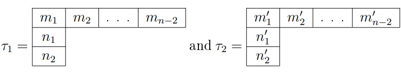 be two
recording row-strict tableaux in \(\mathcal{C}_{n-2,1,1}\). We say \(\tau_{1} \leq \tau_{2}\) if \(m_{i} \geq m'_{i}\) and \(n_{i} \leq n'_{i}\) for \(i=1,2\). Otherwise the tableaux \(\tau_{1}\) and \(\tau_{2}\) are incomparable. We say \(\tau_{2}\) covers \(\tau_{1}\) and write \(\tau_{2}\succ\tau_{1}\) if there does not
exist \(\tau_{3}\in \mathcal{C}_{n-2,
1,1}\) such that \(\tau_{1}<\tau_{3}<\tau_{2}\).
be two
recording row-strict tableaux in \(\mathcal{C}_{n-2,1,1}\). We say \(\tau_{1} \leq \tau_{2}\) if \(m_{i} \geq m'_{i}\) and \(n_{i} \leq n'_{i}\) for \(i=1,2\). Otherwise the tableaux \(\tau_{1}\) and \(\tau_{2}\) are incomparable. We say \(\tau_{2}\) covers \(\tau_{1}\) and write \(\tau_{2}\succ\tau_{1}\) if there does not
exist \(\tau_{3}\in \mathcal{C}_{n-2,
1,1}\) such that \(\tau_{1}<\tau_{3}<\tau_{2}\).
Given a recording row-strict tableau \(\tau \in \mathcal{C}_{n-2,1,1}\), its row-reading, denoted by \(_{\tau}w\), is obtained by listing the row entries of \(\tau\) starting from bottom upward and going from left to right.
Example 4.2. The row reading of 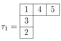 \( \in
\mathcal{C}_{3,1,1}\) is given by \(_{\tau}w =23145\). Notice that \(_{\tau}w\) has a unique descent, therefore,
it is Grassmannian.
\( \in
\mathcal{C}_{3,1,1}\) is given by \(_{\tau}w =23145\). Notice that \(_{\tau}w\) has a unique descent, therefore,
it is Grassmannian.
Remark 4.3. The set \(\mathcal{R}^{_{\tau}w}_{n}\) of row-readings of the recording row-strict tableaux in \(\mathcal{C}_{n-2, 1,1}\) constitutes the Grassmannian permutations whose associated partitions fit into the rectangle \(n-2\times 2\). It is important to point out that these are precisely the indexing permutations of the Schubert varieties inside Grassmannian \({\rm Gr}(2,n)\) of planes in an \(n\)-dimensional complex vector space. In fact, there is a projection \[\label{eq4.1} \pi : \mathcal{F}\ell _{n}({\mathbb{C}})\longrightarrow Gr(2,n), \tag{10}\] from the full flag variety \(\mathcal{F}\ell _{n}({\mathbb{C}})\) to the Grassmannian Gr(2,n) with \(\pi^{-1}(X_{\lambda}(V_{\bullet})) = X_{w(\lambda)}(V_{\bullet})\), where \(X_{\lambda}(V_{\bullet})\) is a Schubert variety in the Grassmannian \(Gr(2,n)\). The permutation \(w(\lambda)\) identified with the partition \(\lambda=(\lambda_{1},\lambda_{2})\) is given by \[\label{eq4.2} w_{i}=i+\lambda_{3-i}, \ 1\leq i\leq 2 \ {\rm and} \ w_{j}< w_{j+1},\ 3\leq j\leq n. \tag{13}\] The reader is referred to [4,7,5,10] for more details on the flag and Grassmannian variety.
Proposition 4.4. Let 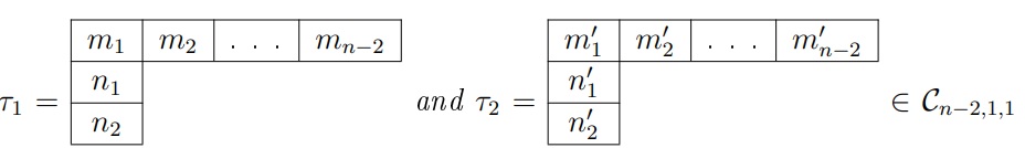 be two recording row strict tableaux.
Then \(\tau_{2}\) covers \(\tau_{1}\) if and only if \(\ell(_{\tau_{2}}w) =
\ell(_{\tau_{1}}w)+1\).
be two recording row strict tableaux.
Then \(\tau_{2}\) covers \(\tau_{1}\) if and only if \(\ell(_{\tau_{2}}w) =
\ell(_{\tau_{1}}w)+1\).
Proof. Suppose that \(\tau_{1}\) covers \(\tau_{2}\), by definition, we have \(\tau_{1} \leq \tau_{2}\), if \(m_{i} \geq m'_{i}\) and \(n_{i} \leq n'_{i}\) for \(i=1,2\) and there does not exist \(\tau_{3}\in \mathcal{C}_{n-2, 1,1}\) such that \(\tau_{1}<\tau_{3}<\tau_{2}\). Thus either \(n_{1}'=n_{1}\) and \(n_{2}'=n_{2}+1\) or \(n_{1}'=n_{1}+1\) and \(n_{2}'=n_{2}\), therefore, \(\ell(_{\tau_{2}}w) = \ell(_{\tau_{1}}w)+1\). On the other hand, consider the two row readings \(_{\tau_{1}}w = n_{1}n_{2}m_{1}\cdots m_{n-2}\) and \(_{\tau_{1}}w = n_{1}'n_{2}'m_{1}'\cdots m_{n-2}'\) in which \(n_{1}<n_{2}>m_{1}<\cdots < m_{n-2}\) and \(n_{1}'<n_{2}'> m_{1}'<\cdots < m_{n-2}'\) such that \(\ell(_{\tau_{2}}w) = \ell(_{\tau_{1}}w)+1\), so either \(n_{1}'=n_{1}\) and \(n_{2}'=n_{2}+1\) or \(n_{1}'=n_{1}+1\) and \(n_{2}'=n_{2}\), hence \(\tau_{2}\) covers \(\tau_{1}\). ◻
There is a natural partial order on the set \(\mathcal{R}^{_{\tau}w}_{n}\) of row-readings of the recording row strict tableaux in \(\mathcal{C}_{n-2, 1,1}\) induced by the Bruhat order on the symmetric group \(\mathfrak{S}_{n}\) described in section 2. Given any two row-readings \(_{\tau_{1}}w, \ _{\tau_{2}}w\in\mathcal{R}^{_{\tau}w}_{n}\), we say \(_{\tau_{1}}w\leq \ _{\tau_{2}}w\) if \(\ell(_{\tau_{1}}w)\leq \ell( _{\tau_{2}}w)\). It is obvious that the Hasse diagram \(\mathcal{H}_{\mathcal{R}^{_{\tau}w}_{n}}\) of the poset \((\mathcal{R}^{_{\tau}w}_{n}, \leq)\) is graded by the permutation length. The maximum element is the permutation \([n-1, n, 1, 2,\dots, n-2]\) while the minimum element is \([1,2,\dots, n]\) since every permutation in \(\mathcal{R}^{_{\tau}w}_{n}\) is Grassmannian described in Eq. 11.
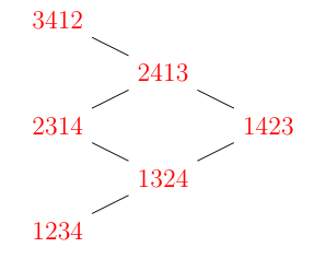
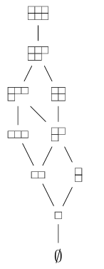
Example 4.5. The Hasse diagram of the poset \((\mathcal{R}^{_{\tau}w}_{4}, \leq)\) is given below
Lemma 4.6. There is an order preserving bijective map between the posets \(( \mathcal{C}_{n-2, 1,1}, \leq)\) and \((\mathcal{R}^{_{\tau}w}_{n}, \leq)\) for \(n\geq 4\).
Proof. It is clear that the map \(\tau\mapsto {_{\tau}w}_{n}\) is a bijection. We only need to show that it is order preserving. Suppose that \(\tau_{1}\leq \tau_{2}\), by Definition 4.1, \(m_{i} \geq m'_{i}\) for \(1\leq i\leq n-2\), \(n_{i} \leq n'_{i}\) for \(1\leq i\leq 2\), and \(1\leq n_{i} , n'_{i}, m_{i} , m'_{i}\leq n\) so that \(_{\tau_{1}}w = [ n_{1},n_{2},m_{1},\cdots , m_{n-2}]\) such that \(n_{1}<n_{2}>m_{1}<\cdots < m_{n-2}\) and \(_{\tau_{2}}w=[n_{1}',n_{2}', m_{1}',\cdots , m_{n-2}']\) such that \(n_{1}'<n_{2}'> m_{1}'<\cdots < m_{n-2}'\). Notice that \(\ell(_{\tau_{1}}w)\leq \ell( _{\tau_{2}}w)\), therefore, \(_{\tau_{1}}w\leq \ _{\tau_{2}}w\). ◻
Theorem 4.7. The Hasse diagram \(\mathcal{H}_{\mathcal{C}_{n-2, 1,1}}\) of the poset \(( \mathcal{C}_{n-2, 1,1}, \leq)\) is graded, with rank function \(\rho\) defined by the permutation length, \(\displaystyle\rho(\tau) = \ell({_\tau}w)\) for every \(\tau\in \mathcal{C}_{n-2, 1,1}\) where \({_\tau}w\) is the row-reading of \(\tau\). Furthermore, \(\mathcal{C}_{n-2, 1,1}\) is of the rank \(\displaystyle2(n-2).\)
Proof. It is straightforward to see that the graded structure of the Hasse diagram \(\mathcal{H}_{\mathcal{C}_{n-2, 1,1}}\) of \(( \mathcal{C}_{n-2, 1,1}, \leq)\) is realised by identifying it with the Hasse diagram \(\mathcal{H}_{\mathcal{R}^{_{\tau}w}_{n}}\) of its corresponding poset \((\mathcal{R}^{_{\tau}w}_{n}, \leq)\) of row-readings of the recording row-strict tableaux. The maximum element is the row-strict tableau \(\tau'\) whose reading \(_{\tau'}w\) is the permutation \([n-1, n, 1, 2,\dots, n-2]\) while the permutation of the minimum element \(\tau\) is \(_{\tau}w=[1,2,\dots, n]\). The length \(\ell(_{\tau'}w)\) of the permutation \(_{\tau'}w\) associated to the maximum element \(\tau'\) is \(2(n-2)\), hence the rank of the poset. ◻
Corollary 4.8. There is a chain of isomorphisms between the graph \(\mathcal{G}_{_{n}w}\) of reduced words of the permutation \(_{n}w\), the Hasse diagram \(\mathcal{H}_{\mathcal{C}_{n-2, 1,1}}\) of the poset \(( \mathcal{C}_{n-2, 1,1}, \leq)\) and the Hasse diagram \(\mathcal{H}_{\mathcal{R}^{_{\tau}w}_{n}}\) of the poset \((\mathcal{R}^{_{\tau}w}_{n}, \leq)\).
More is true about the chain of isomorphisms in Corollary 4.8. The identification of the graph \(\mathcal{G}_{_n{w}}\) with the Hasse diagrams \(\mathcal{H}_{\mathcal{C}_{n-2, 1,1}}\) and \(\mathcal{H}_{\mathcal{R}^{_{\tau}w}_{n}}\) reveals a fundamental connection between the graph of reduced words and the lattice point graph \(\mathcal{G}_{(n-2)\Delta_{2}}\) of \((n-2)\)-fold dilation of the standard 2- simplex \(\Delta_{2}\) . Recall that the standard \(2\)-simplex \(\Delta_2\) is the convex hull of the set \(\{\underline{0}, e_1,e_2\}\) where \(e_1, e_2\) are the standard vectors in \({\mathbb{R}}^{2}\) and \(\underline{0}\) is the origin. That is, \[\label{eq5.1} \Delta_{2}:= \{{\bf x}\in{\mathbb{R}}^{2} : {\bf x}\cdot e_{i}\geq 0, \ \ \sum_{i=1}^{2} {\bf x}\cdot e_{i}\leq 1\}, \tag{12}\] and the dilation \(k\Delta_{2}\), is given by \[\label{eq5.2} k\Delta_{2}=\{{\bf x}\in{\mathbb{R}}^{2} :{\bf x}\cdot e_{i}\geq 0, \ \ \sum_{i=1}^{2}{\bf x}\cdot e_{i}\leq k\}. \tag{13}\]
The standard 2- simplex \(\Delta_{2}\) is a lattice polytope. Counting the lattice points of any given lattice polytope is the central theme of the Ehrhart theory [2,1,13,10]. In fact, the number of the lattice points on \(k\Delta_2\) is given by the Ehrhart polynomial \[\label{eq5.3} \mathcal{L}_{\Delta_{2}}(k)=|k\Delta_{2}\cap {\mathbb{Z}}_{\geq 0}^{2}|= {{k+2}\choose 2}. \tag{14}\]
Our interest is in the graph \(\mathcal{G}_{k\Delta_{2}}\) of the set \(\mathcal{C}:= k\Delta_{2}\cap {\mathbb{Z}}_{\geq 0}^{2}\) of lattice points on \(k\Delta_{2}\). Notice that the elements of \(\mathcal{C}\) are the integer solutions of the inequality \[\label{eq5.4} \sum_{i=1}^{2}{\bf x}\cdot e_{i}\leq k. \tag{15}\]
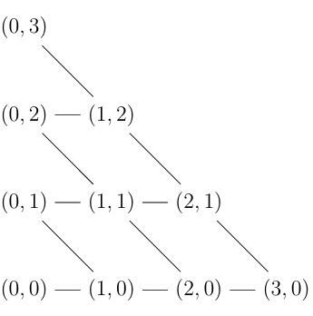
In order to construct the graph we define a lexicographical order \(<_{\rm lex}\) on the elements of \(\mathcal{C}\) as follows: Let \({\bf a}=(a_1,a_2)\) and \({\bf b}=(b_1,b_2)\) be any two lattice points in \(\mathcal{C}\). We say \({\bf a} <_{\rm lex} {\bf b}\) if in the integer coordinate difference \({\bf a}-{\bf b}\in{\mathbb{Z}}^{2}\), the first coordinate is negative. The order induces a directed graph \(\stackrel{\rightarrow}{\mathcal{G}_{k\Delta_{2}}}\) whose vertices are given by the elements of the set \(\mathcal{C}\) such that there is an edge between \({\bf a} \ {\rm and}\ {\bf b}\) in \(\mathcal{C}\) if \({\bf b} \ {\rm covers}\ {\bf a}\) and write \({\bf a}\lessdot{\bf b}\), that is, there does not exist a lattice point \({\bf c}\in \mathcal{C}\) such that \({\bf a}<_{\rm lex} {\bf c}<_{\rm lex}{\bf b}\). The sub-lattice graph \(\mathcal{G}_{k\Delta_2}\) is the underlying graph of the digraph \(\stackrel{\rightarrow}{\mathcal{G}_{k\Delta_{2}}}\), that is, the graph containing undirected edges in which all edge fibers are identical. For instance, the sub-lattice graph \(\mathcal{G}_{3\Delta_2}\) is given in Figure 7 below.
There is no edge between any pair of vertices of \(\mathcal{G}_{k\Delta_2}\) if they share the first coordinates. By setting \(k\) to be \(n-2\), it turns out that the vertices of the graph \(\mathcal{G}_{k\Delta_2}\) of lattice points in \(\mathcal{C}\) encode the fitted partitions associated with the Grassmannian permutations which constitute the vertices of the Hasse diagram \(\mathcal{H}_{\mathcal{R}^{_{\tau}w}_{n}}\) of the poset \((\mathcal{R}^{_{\tau}w}_{n}, \leq)\) described in the Remark 4.3. To see this we associate to each lattice point \({\bf a}=(a_1,a_2)\in \mathcal{C}\), a weight \({\bf m}_{\bf a}\) given by \[\label{eq5.5} {\bf m}_{\bf a} = \sum_{t=1}^{2} ta_{t}, \tag{16}\] and partition \(\lambda = (\lambda_1, \lambda_2)\vdash {\bf m}_{\bf a}\). Notice that \({\bf m}_{\bf a}= (1,2)\cdot{\bf a} = {\bf m}_{\bf a}\) for a fixed vector \((1,2)\) so that \(\lambda_{1} = a_{1}+a_{2}\) and \(\lambda_{2} =a_{2}\).
Proposition 5.1. Let \({\bf a}=(a_1,a_2)\) be a lattice point in \(\mathcal{C}\) such that \({\bf m}_{\bf a}\) and \(\lambda=(\lambda_1,\lambda_2)\) are respectively the weight and the partition associated with \({\bf a}\). Then \(\lambda\) is a partition of \({\bf m}_{\bf a}\) which fits into the rectangle \(\square_{k\times 2}\).
We now give the poset associated to the fitted partitions associated with the lattice points in \(\mathcal{C}\). The concept of fitted partitions as well as their ordering is well-known in Schubert calculus. These partitions index Schubert varieties of the Grassmannian variety, see [7,5] for more details on partitions indexing Schubert varieties of the Grassmannian. Let \(\mathcal{C}_{\square_{k\times 2}}\) be the set of fitted partitions in the rectangle \(\square_{k\times 2}\), the partial order on \(\mathcal{C}_{\square_{k\times 2}}\) is given as follows; for \(\lambda=(\lambda_{1},\lambda_{2}), \mu=(\mu_{1},\mu_{2})\in \mathcal{C}_{\square_{k\times 2}}\), we say \(\lambda\leq\mu\) if \(\lambda_{i}\leq\mu_{i}\), for \(i=1,2\). This gives rise to the Young’s lattice \(\mathcal{Y}_{\mathcal{C}_{\square_{k\times 2}}}\) on the corresponding Young diagrams. It is graded since the rank function is given by the number of boxes in each of the diagrams.
Example 5.2. The Young’s lattice of \(\mathcal{C}_{\square_{3\times 2}}\) is given by
Now, for a fixed vector \({\bf z}=(1,2)\), consider the set
\[N^{\bf z}_{{\bf m}_{\bf a}} = \#\{ {\bf a} \in k\Delta_{2}\cap {\mathbb{Z}}_{\geq 0}^{2} : {\bf a}\cdot {\bf z} = {\bf m}_{\bf a} \}.\]
Geometrically, it means the simplex \(k\Delta_{2}\) is being sliced by the line segments \(a_1 +2a_2 = {\bf m}_{\bf a}\) and the lattice points of \(k\Delta_{2}\) on each of these lines are being counted. This is deeply connected with graded Ehrhart theory. The reader is referred to [2,1] for more information on refined Ehrhart theory. Notice that \(0\leq {\bf m}_{\bf a}\leq 2k\) so that the graded polynomial \({\rm P}^{\bf z}_{k}(q)\) is given by \[\label{eq5.6} {\rm P}^{\bf z}_{k}(q)= \sum_{{\bf m}_{\bf a}=0 }^{2k} N^{\bf z}_{{\bf m}_{\bf a}} q^{{\bf m}_{\bf a}}= \left[ k+2 \choose 2\right]_q \tag{17}\] with the product expansions given given by \[\label{eq5.7} {\rm G}(q,t) = \prod^{2}_{i=0}\frac{1}{(1-q^{i}t)}. \tag{8}\]
The graded polynomial \({\rm P}^{\bf z}_{k}(q)\) is a refinement of the Ehrhart polynomial \(\mathcal{L}_{\Delta_{2}}(k)\) of the \(k\)-fold dilation of the standard 2-simplex. Therefore, the Hasse diagram \(\mathcal{G}_{k\Delta_2}\) of the poset \((k\Delta_{2}\cap {\mathbb{Z}}_{\geq 0}^{2}, <_{\rm lex})\) is graded with rank function \(\rho({\bf a})={\bf m}_{\bf a}\) where \((0, k)\) and \((0,0)\) are respectively the maximum and minimum elements. In fact, its rank polynomial is in Eq. (17). This is deeply connected with the Poincaré polynomial of the cohomology \({\rm H}^{\ast}({\rm Gr}(2,n), {\mathbb{Z}})\) of the Grassmannian of 2-planes in the 4-complex space, that is, the Hilbert series for a graded ring arising from the Borel presentation of the cohomology ring [7]. It is well-known that to every fitted partition \(\lambda\subseteq\square_{k\times2}\) there is a corresponding Grassmannian permutation \(w(\lambda)\) given in Eq. (11) [7,5]. These permutations, denoted by \(\mathcal{R}^{_{\tau}w}_{n}\), are precisely the row-readings of the set \(\mathcal{C}_{n-2,1,1}\) of recording row-strict tableaux \(\tau\) in which the tableaux encode the positions of descents and ascents of the vertices of the graph \(\mathcal{G}_{_{n}w}\) of reduced words of the permutation \(_{n}w\).
Proposition 5.3. Let \({\bf a}=(a_1,a_2)\) be a lattice point in \(\mathcal{C}\) such that \({\bf m}_{\bf a}\) and \(\lambda=(\lambda_1,\lambda_2)\) are respectively the weight and the partition associated with \({\bf a}\). Then the length of the Grassmannian permutation \(w(\lambda)\in\mathcal{R}^{_{\tau}w}_{n}\) corresponding to \(\lambda\) is \({\bf m}_{\bf a}\).
Proof. Since the Grasmmannian permutation \(w(\lambda)\) is of the form \[w_{i}=i+\lambda_{3-i}, \ 1\leq i\leq 2 \ {\rm and} \ w_{j}< w_{j+1},\ 3\leq j\leq n,\] so its Lehma code \(c(w(\lambda))\) is given by \((w_{1}-1, w_{2}-2, 0,\dots,0)\). The sum of the entries of the code is the length of the permutation since each entry in the \(i^{th}\) coordinate by definition denotes the number of inversions associated with the value \(w_{i}\) of the permutation. The non-increasing rearrangement of nonzero entries of the code \(c(w(\lambda))\) is precisely the partition \(\lambda\), hence, \[w_{2} +w_{1}-3 =\ell(w(\lambda)) = \lambda_1 +\lambda_2 = {\bf m}_{\bf a}\] ◻
The projection \(\pi\) in the Eq. (10) induces a monomorphism \(\pi^{\ast}\) at the level of cohomology. \[\label{eq5.8} \pi^{\ast} :{\rm H}^{\ast} ({\rm Gr}(2,n), {\mathbb{Z}}) \longrightarrow {\rm H}^{\ast}(\mathcal{F}\ell _{n}({\mathbb{C}}),{\mathbb{Z}}) , \tag{19}\] which takes cycle \(\sigma_{\lambda}\) to the cycle \(\sigma_{w(\lambda)}\). The reader is referred to [7,5] .The cohomology ring of the Grassmannian \(Gr(2,n)\) is generated by the Schubert cycles \(\sigma_{\lambda}\). These are Poincaré dual of the fundamental classes in the homology of Schubert varieties. The ring is isomorphic to the coinvariant algebra via Borel presentation, that is, \[\label{eq5.9} {\rm H}^{\ast} ({\rm Gr}(2,n), {\mathbb{Z}})\cong \frac{{\mathbb{Z}}[x_1,\dots, x_n]^{\frak{S}_{2}\times\frak{S}_{n-2}}}{{\mathbb{Z}}^{+}[x_1,\dots,x_n]^{\frak{S}_{n}}}. \tag{20}\]
Therefore, the Hilbert series of the coinvariant algebra is the Poincaré polynomial of the cohomology ring, that is, the Gaussian polynomial \(f(t)\) given by \[\label{eq5.10} f(t)=\frac{(1-t^{n})(1-t^{n-1})}{(1-t)(1-t^2)}. \tag{21}\] Notice that this is precisely the rank polynomial given in Eq. (17). The reader is referred to [7] for more detail on the Hilbert-Poincaré series of the cohomology ring of Grassmannian and flag variety.
Proposition 5.4. Setting \(k=n-2\), there is an order preserving between the posets \((k\Delta_{2}\cap {\mathbb{Z}}_{\geq 0}^{2}, <_{\rm lex})\) and \((\mathcal{R}^{_{\tau}w}_{n}, \leq)\) making the Hasse diagrams \(\mathcal{G}_{k\Delta_2}\) and \(\mathcal{H}_{\mathcal{R}^{_{\tau}w}_{n}}\) isomorphic.
Corollary 5.5. The following chain of isomorphisms holds \[\mathcal{G}_{_{n}w}\cong \mathcal{H}_{\mathcal{C}_{n-2, 1,1}}\cong \mathcal{H}_{\mathcal{R}^{_{\tau}w}_{n}}\cong \mathcal{Y}_{\mathcal{C}_{\square_{(n-2)\times 2}}}\cong\mathcal{G}_{(n-2)\Delta_2}, \ n\geq 4.\]
Example 5.6. Consider the set \(\mathcal{C}:= 3\Delta_{2}\cap {\mathbb{Z}}_{\geq 0}^{2}\) of lattice points on the \(3\)-fold dilation of the standard 2-simplex \(\Delta_2\). That is, \[\mathcal{C}=\{ (0,3), (1,2), (0,2), (2,1), (1,1), (3,0), (0,1), (2,0), (1,0), (0,0) \}.\]
The set \(\mathcal{C}_{\lambda}\) of
the corresponding fitted partitions \(\lambda\subseteq\square_{3\times 2}\) is
given by \[\mathcal{C}_{\lambda}= \{ (3,3),
(3,2), (2,2), (3,1), (2,1]), (3), (1,1), (2), (1), \emptyset
\},\] thus, the set \(\mathcal{C}_{w(\lambda)}\) of the
corresponding Grassmannian permutations is given by \[\mathcal{C}_{w(\lambda)}=\{45123, 35124, 34125,
25134, 24135, 15234, 23145, 14235, 13245,
12345\}=\mathcal{R}^{_{\tau}w}_{5}\]
 \[\mathcal{G}_{_{n}w}= \{ 432134, 432314, 432341,
423214, 423241, 243214, 423421, 243241, 243421, 234321\}\]
\[\mathcal{G}_{_{n}w}= \{ 432134, 432314, 432341,
423214, 423241, 243214, 423421, 243241, 243421, 234321\}\]
I would like to thank Balazs Szendroi, Ben Young, and Mike Zabrocki for productive discussions during the preparation of the manuscript. The anonymous referee is highly appreciated for the useful suggestions and comments to improve the presentation significantly.