
Target detection is an important task in computer vision, whose goal is to detect and localize the target objects of interest from images or videos, and is widely used in medical imaging and automatic driving and other fields. For example, in automatic driving, target detection algorithms can be used to monitor the road surface in real time, distinguish objects such as pedestrians and trees, and help the system make accurate judgments [23,8]. This is different from image classification, target detection not only needs to determine whether there is a specific object in the image, but also needs to accurately label the location of the object. Target detection algorithms are categorized into two schools of thought: traditional algorithms and deep learning-based algorithms [14,11]. Traditional algorithms rely on hand-designed features and cumbersome processes, while deep learning methods show significant performance improvement in the target detection task through end-to-end learning of feature representations, especially in dealing with complex scenes and large-scale datasets. Therefore, deep learning-based algorithms have now become the mainstream of target detection [26,24]. Deep learning-based target detection algorithms are categorized into two-stage algorithms (e.g., R-CNN series) and single-stage algorithms (represented by YOLO). Two-stage algorithms improve the accuracy by generating candidate regions and two stages of classification and localization, and single-stage algorithms realize one-time completion of classification and localization by transforming the detection task into a regression problem, and representative algorithms include YOLO [27,12]. YOLO is to transform the target detection problem into a regression problem, thus realizing a detection method from end to end. Compared with the traditional two-stage target detection algorithm, the single-stage target detection algorithm has a great improvement in speed, thus realizing the balance between speed and accuracy [20,10].
In this paper, based on the YOLOv5 framework, data enhancement techniques are used in the input of the target detection model to improve the robustness and generalization ability of the model. In the target detection task, the function of adaptive scaling image is added to improve the detection speed to some extent. The output part mainly adopts the complete intersection and ratio loss function, which improves the accuracy of the model calculation. The C3_Attention module is utilized to replace the C3 module in the original YOLOv5s backbone network to fully integrate the attention mechanism with the YOLOv5s network model. Two metrics, precision rate and recall rate, are chosen to evaluate the performance and efficiency on the target detection task.
Convolutional neural network is a deep learning model with its own convolutional structure, which effectively reduces the complexity of the network with local sensory fields and weight sharing, making the network easier to train. Taye [17] describes the building blocks, roles and uses of Convolutional Neural Networks (CNNs), aiming to help academics understand the research gaps that exist in the field of Convolutional Neural Networks. Carata et al. [2] designed a yolo deep neural network model for use in the dark web framework to understand how the neural network makes certain decisions regarding the final prediction outcome and experimentally verified the effectiveness of the model, which generates and displays a feature map of any point in the network. Du and Jiao [7] proposed a lightweight convolutional neural network model for enhanced feature extraction based on the YOLO algorithm, which was applied to the existing highway traffic road pothole defects detection, and its superior performance was verified through the model evaluation test, which can detect the pavement defects problem well. Huang et al. [9] highlights the wide range of applications of YOLO neural networks in the field of computer vision and proposes an FPGA-based YOLO neural network design space exploration method, which can improve the efficiency of the convolutional operations, which in turn can greatly improve the speed of the neural network. Dewi et al. [5] measured two models, Yolo V4 and Yolo V4-tiny merged Spatial Pyramid Pool (SPP), and analyzed the optimal performance of Yolo V4_1 (with SPP), and therefore developed a deep convolutional neural network based on this to enhance traffic sign recognition in order to facilitate real-time traffic sign detection in real-world autonomous driving scenarios. Zhang et al. [28] expresses the fact that deep learning has been successfully applied in the field of feature extraction and classification of hyperspectral images, and in order to solve the problems existing at this stage of target detection in hyperspectral images, a new deep convolutional neural network (HTD-Net) is designed, and experimental results derived from the use of several real hyperspectral data demonstrate the advantages of the proposed algorithm over the traditional target detectors.
Target detection technology occupies a pivotal position in the field of artificial intelligence, and it is a challenging task in computer vision research. Wen et al. [21] reviews the development history of YOLO algorithm and its application in the field of target detection, takes the current latest YOLOv5 algorithm as an example, studies its main framework and main content, and evaluates its detection effect through practical recognition and detection applications. Tan et al. [16] designed a multi-target tracking algorithm based on YOLO, and verified the effectiveness and practicability of the designed algorithm through experiments on the public target tracking dataset MOT-16 and MSR dataset, which can improve the accuracy and efficiency of multi-target tracking. Li et al. [13] developed a multi-target detection and tracking algorithm combined with YOLO v3 to solve the occlusion problem in the current video multi-target tracking process, and the superior performance of the developed algorithm is verified through experimental tests, which can track the occluded targets in the test video more accurately. Zhou et al. [29] proposed an improved detection algorithm YOLO-SASE based on the YOLO detection framework and SRGAN network that can enhance the detection of infrared small targets in complex backgrounds, and the proposed algorithm demonstrated high accuracy, recall and stability in the comparison experiments with the original model. Yan et al. [25] proposed a lightweight target detection method based on the improved YOLOv5s and applied it to an apple picking robot, and the empirical analysis verified the effectiveness of the proposed improved method in recognizing graspable apples that are not occluded by leaves or only occluded by leaves, as well as non-graspable apples that are occluded by branches or occluded by other fruits. Wu et al. [22] combines local full convolutional neural network and YOLO v5 algorithm and applies it to small target detection in remote sensing images, the experimental results affirm the feasibility of this initiative, which can achieve more accurate feature recognition and detection performance, and provide reference value for the application of remote sensing technology in China. Chen et al. [3] designed an underwater-YCC optimization algorithm based on YOLO v7 for the phenomenon that fuzzy distortion and irregular light absorption in underwater environments often lead to image blurring and color deviation, and verified the superior detection performance of this algorithm through several experiments, which can improve the detection accuracy of underwater small targets. Han et al. [6] discussed the target detection method based on CNN system and YOLO, and pointed out that YOLO is one of the best representatives of CNN, which can innovate a brand new method to solve the object detection in the simplest and the most efficient way, with a strong generalization ability, and achieves an excellent trade-off between speed and accuracy.
Deep learning-based target detection algorithms have benefited from the birth of neural networks (NNs), which can automatically acquire useful feature information in images by learning from a large number of datasets, thus avoiding the manual extraction of features in traditional target detection [15]. As early as the 1940s, researchers for artificial neural networks (ANN) exploration has been carried out, this mathematical model simulates the human brain’s nervous system to deal with the processing mechanism of external information, and its basic structure and the human brain’s nervous system information processing mechanism is similar.
As scholars’ research on neural networks continues to deepen, it is found that with the increasing number of hidden layers, it is more difficult to train the fully connected weights in BP neural networks, which requires a larger dataset capacity. In this case, Convolutional Neural Networks (CNNs) came into being, and the birth of CNNs also laid an important foundation for a series of deep learning target detection algorithms today.
Convolutional neural network is a special kind of feed-forward neural network, whose most distinctive feature is the structure with weight sharing and sparse connectivity [18]. It usually consists of an input layer, a convolutional layer, a pooling layer, a fully connected layer and an output layer.
Figure 1 shows the linear and nonlinear problems, the activation function is an important part of the neural network, in the convolutional neural network, each layer of the output obtained in the neuron node transmission between the neuron nodes can only be processed for the linear mapping, in this case, even more hidden layers can not change the overall network is equivalent to the nature of a single-layer neural network, and this will also lead to a number of nonlinear problems can not be solved as shown in the figure on the left. As shown in the figure, the left figure is a linearly divisible problem, but also one of the simplest binary classification problem, while the right figure is a linearly indivisible nonlinear problem, this time it is necessary to divide into a nonlinear curve to classify, and the activation function is the key to facilitate this nonlinear classification.
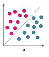
Therefore, it is necessary to introduce activation functions in neural networks to provide nonlinear modeling capabilities. Activation functions enable deep neural networks to achieve hierarchical nonlinear mapping learning for better handling of complex input data. Activation functions should usually be characterized by properties such as differentiability and monotonicity, and common activation functions include the following:
The Sigmoid function is one of the very common activation functions, as can be seen from the figure, the value domain of its curve is \(\left(0,1\right)\), and the value of the curve converges infinitely to 1 and 0, respectively, as \(x\) continues to increase and decrease, and its functional expression is: \[\label{GrindEQ__1_} f_{sigmoid} \left(x\right)=\frac{1}{1+e^{-x} } . \tag{1}\]
The Tanh function is a hyperbolic tangent function, as can be seen from the figure the Tanh function has a very similar function curve to the Sigmoid function, and its functional expression is: \[\label{GrindEQ__2_} f_{\tanh } \left(x\right)=\frac{e^{x} -e^{-x} }{e^{x} +e^{-x} } . \tag{2}\]
ReLU is a linear rectification function, also known as linear correction unit, whose functional expression is: \[\label{GrindEQ__3_} f_{RCLU} \left(x\right)=\left\{\begin{array}{l} {x,x\ge 0}, \\ {0,x<0}. \end{array}\right. \tag{3}\]
The Leaky ReLU function is characterized by the possibility of solving the zero gradient problem for negative values by giving very small linear components to negative inputs, and its helps to extend the functional range of ReLU, which is calculated as: \[\label{GrindEQ__4_} f_{LeakyReLU} \left(x\right)=\left\{\begin{array}{l} {x,x>0}, \\ {\alpha x,x\le 0} .\end{array}\right. \tag{4}\]
YOLOv5 target detection algorithm was proposed in 2020, which added new algorithmic ideas on the basis of YOLOv4 algorithm, and greatly improved its accuracy and speed [4]. There are four versions of the official model of YOLOv5, which are YOLOv5s, YOLOv5m, YOLOv51, and YOLOv5x with different sizes of models, and analyzed as a whole, each different size model has the same network structure distribution. Each model of different sizes has the same network structure distribution, and the following is a brief introduction to the three main structural components of the YOLOv5 algorithm.
The input side of YOLOv5 adopts various data enhancement techniques to improve the robustness and generalization ability of the model, mainly including:
Similar to YOLCM, mosaic data augmentation is still used in the input of YOLOv5, however, the main idea is to stitch four randomly cropped images onto one image as the training image, the dataset is enriched in this way, and the robustness of the network is better.
Anchor frame is a commonly used method in target detection which captures targets of different sizes and proportions by defining multiple predefined frames of different sizes and proportions in the image. Therefore, in the previous YOLO series of algorithms different datasets are initially set with fixed length and width anchor frames. During the training process, the algorithm would output a predicted frame based on the initially set anchor frame, compare it with the real frame, calculate the intersection ratio between the two, and then iteratively update it in reverse. The adaptive anchor frame technology no longer hard-codes the size and ratio of each preset anchor frame, but instead adaptively obtains the optimal anchor frame size and ratio from the input training data through the clustering algorithm, which makes it possible to adaptively compute the optimal anchor frame values in different training sets for each training, which reduces the subjectivity and uncertainty in the design of anchor frames, and improves the accuracy and generalization ability of the detection model.
In the target detection task, the size of the input image has an important impact on the results output by the model. If the input image is too small, it will result in the model not being able to detect small targets well or locate the target’s edges inaccurately, while if the input image is too large, it will increase the computational burden and reduce the speed and efficiency of the model. In the YOLOv5 algorithm, the function of adaptive image scaling is added, which makes the size of the short edges of the scaled image within a certain range, which makes the problem of different sizes of the black edges due to different aspect ratios of the images be solved, and also reduces the amount of computation when reasoning about the images, which improves the detection speed to a certain extent.
The output part of YOLOv5 mainly adopts the full intersection and merger ratio loss function. The initial intersection and merger ratio loss function only takes the overlapping area of the detection frame and the target frame into consideration, which ignores the problem of the different relative positions when the detection frame and the target frame do not overlap. To address this point, the generalized intersection and merger ratio loss function (GIoU_Loss) function was proposed, which notates the value of IoU_Loss as \(F_{IoU\_ Loss}\), and the value of GIoU_Loss as \(F_{GIoU\_ Loss}\) its calculation formula is [19]: \[\label{GrindEQ__5_} F_{CIoU\_ Loss{\rm \; }} =F_{IoU\_ Loss} -\frac{C-A\cup B}{C} , \tag{5}\] where \(A\) and \(B\) represent the detection frame and the target frame, respectively, and \(C=A\cap B\). The distance intersection and merging ratio loss function (DIoU_Loss), on the other hand, adds the computation of the distance between the target frame and the center point of the detection frame on the basis of the previous two, which solves the regression inaccuracy problem that occurs when the target frame wraps the detection frame. The Euclidean distance between the target frame and the detection center point is denoted as \(F_{Dis\tan ce\_ 2}\), the diagonal distance between the target frame and the smallest outer rectangle of the detection frame is denoted as \(F_{Dis\tan ce\_ C}\), and DIoU_Loss is denoted as \(F_{DIoU\_ Loss}\), which gives its calculation formula: \[\label{GrindEQ__6_} F_{DIoU\_ Loss} =1-\left(F_{IoU\_ Loss} -\frac{F_{Dis\tan ce\_ 2} {}^{2} }{F_{Dis\tan ce\_ C} } \right) . \tag{6}\]
According to the calculation method of the DIoU_Loss function, the CIoU_Loss function used in YOLOv5 then adds an influence factor to take the aspect ratio of the target frame and the prediction frame into account, and marks the CIoU_Loss as \(F_{IoU\_ Loss}\), and its calculation formula is: \[\label{GrindEQ__7_} F_{CIoU\_ Loss} =1-\left(F_{IoU\_ Loss} -\frac{d_{0}^{2} }{d_{c}^{2} } -\frac{v^{2} }{1-F_{IoU\_ Loss} +v} \right) , \tag{7}\] where \(d_{0}\) is the Euclidean distance between the target frame and the center point of the prediction frame, \(d_{c}\) is the distance between the diagonals of the target frame, and \(v\) is a parameter that measures the aspect ratio, defined by Eq: \[\label{GrindEQ__8_} v=\frac{4}{\pi ^{2} } \left(\arctan \frac{w^{gt} }{h^{g} } -\arctan \frac{w^{p} }{h^{p} } \right)^{2} , \tag{8}\] where \(w^{gt}\) and \(h^{gt}\) correspond to the width and height of the real target frame, and \(w^{p}\) and \(h^{p}\) correspond to the width and height of the predicted frame, respectively. The CIoU_Loss function further takes into account the influencing factors such as overlapping area, center distance and aspect ratio, which makes the calculation of the loss function more accurate.
According to the different principles of action of the attention mechanisms, some of the current advanced attention mechanisms can be classified into six categories: channel attention, spatial attention, temporal attention, branching attention, mixed channel and spatial attention, and mixed spatial and temporal attention [1]. In this paper, we have selected the typical attention methods to be introduced in detail, and we will incorporate this attention mechanism into the YOLOv5 network model to construct a new network model in the subsequent work.
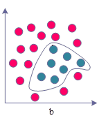
The average pooling of the input feature maps along the two directions of width and height is done respectively in CA, and the position information is embedded into the channel attention, so as to achieve the effect of obtaining both channel attention and spatial attention at the same time.The structure of CA is shown in Figure 2.
As can be seen from the structure diagram, the input feature maps are first average pooled along the height direction and width direction, respectively, with the expression: \[\label{GrindEQ__9_} z^{h} =\frac{1}{W} \sum _{0\le i<W}x \left(h,i\right) , \tag{9}\] \[\label{GrindEQ__10_} z^{w} =\frac{1}{H} \sum _{0\le j<H}x \left(j,w\right) , \tag{10}\] where \(x\) is the input feature map, \(x\in {\rm R}^{C\times H\times W}\), \(z^{h}\) are the outputs after average pooling along the height direction, \(z^{h} \in {\rm R}^{C\times H\times 1}\), \(z^{w}\) are the outputs after average pooling along the width direction, and \(z^{w} \in {\rm R}^{C\times 1\times W}\). The two outputs obtained are then spliced along the channel direction, and the outputs are activated by a two-dimensional convolution, a one-time batch normalization, and a one-time nonlinear function with the expression: \[\label{GrindEQ__11_} f=\delta \left(BN\left(Conv2d^{1\times 1} \left(z^{h} ,z^{w} \right)\right)\right) , \tag{11}\] where \(Conv2d^{1\times 1}\) denotes a 2D convolution with a convolution kernel size of 1 \(\mathrm{\times}\) 1, \(BN\) denotes a batch normalization operation, \(\delta\) is a nonlinear activation function, \(f\) is an intermediate output feature map, and \(f\in {\rm R}^{{C\mathord{\left/ {\vphantom {C r}} \right. } r} \times 1\times \left(H+W\right)}\). \(r\) is used to control the channel reduction rate as in the SE block. Then \(f\) is split into two independent tensors \(f^{h}\) and \(f^{w}\), \(f^{h} \in {\rm R}^{C\times H\times 1}\), \(f^{w} \in {\rm R}^{C\times 1\times W}\), and these two tensors are subjected to 2D convolution and Sigmoid function activation respectively to output two attentions \(g^{h}\) and \(g^{w}\), \(g^{h} \in {\rm R}^{C\times H\times 1}\), \(g^{w} \in {\rm R}^{C\times 1\times W}\). Finally, these two attentions are multiplied by the original inputs \(x\) to obtain the final feature maps outputs \(y\), \(y\in {\rm R}^{C\times H\times W}\), which are expressed as: \[\label{GrindEQ__12_} f^{h} ,f^{w} =Split\left(f\right) , \tag{12}\] \[\label{GrindEQ__13_} g^{h} =\sigma \left(Conv2d^{1\times 1} \left(f^{h} \right)\right) , \tag{13}\] \[\label{GrindEQ__14_} g^{w} =\sigma \left(Conv2d^{1\times 1} \left(f^{w} \right)\right) , \tag{14}\] \[\label{GrindEQ__15_} y=g^{h} \cdot g^{w} \cdot x , \tag{15}\] where Split is the split tensor and \(\sigma\) is the Sigmoid function.
CA is also a hybrid channel and spatial attention mechanism, but it innovatively embeds spatial information into channel information. Due to its lightweight design and flexibility, it can be easily used in classical building blocks for mobile networks. Experiments demonstrate that CA not only helps in image classification but also performs better in downstream tasks such as target detection and semantic segmentation.
More and more studies have shown that an efficient attention mechanism can significantly improve the performance of convolutional neural networks with little additional computational cost added, so it is a very feasible solution to introduce an attention mechanism into YOLOv5 to improve its target detection performance. In this paper, we propose to use YOLOv5s as the base model and insert the CA attention mechanism into YOLOv5s network to construct a new network model to improve the target detection accuracy of YOLOv5s.
There are four C3 modules in the backbone network of YOLOv5s, and each C3 module contains a different number of BottleNecks, which are 1, 2, 3 and 1. In order to facilitate the differentiation and subsequent research, these four positions are numbered according to the order from the shallow network to the deep network, which are called P1, P2, P3 and P4.
Among the convolutional neural networks, the features extracted by the shallow network are closer to the input and contain more pixel information, mainly fine-grained information, such as color, texture, edge, and corner information. The features extracted by the deep network are farther away from the input and contain more abstract information, i.e., semantic information, mainly coarse-grained information. Therefore, in order to improve the feature extraction ability of YOLOv5s, and to be able to fully enhance the effective features while suppressing the background noise, this paper utilizes the C3_Attention module to replace all four C3 modules in the original YOLOv5s backbone network, fully integrates the attention mechanism with the YOLOv5s network model, and constructs the YOLOv5s network model that integrates the attention mechanism.
The YOLOv5 network uses a mean-variance loss function. Since target detection contains two tasks, localization and classification, it is necessary to distinguish between localization error and classification error, and different weight values need to be used for different parts. The algorithm uses relatively large weights for the localization error, i.e., the bounding box coordinate prediction error. And for the classification error a relatively small weight value is used.
Each cell in the network design needs to predict multiple bounding boxes, but its corresponding category is only one. Thus, during the network training process, if a target does exist in the current cell, only the bounding box with the largest \(IoU\) to the actual target is selected to be responsible for predicting the target, while the other bounding boxes are considered to have no target. This setup will enable the corresponding bounding boxes of a cell to apply to targets of different sizes and dimensions respectively. This improves the detection accuracy of the network. The classification error term is computed only if a target does exist in a cell, otherwise the term cannot be computed and is meaningless. The loss function for YOLOv5 network training is shown in Eq. (16):
\[\begin{aligned} \label{GrindEQ__16_} \text{loss} &= \lambda_{\text{coord}} \sum_{i=0}^{S^2} \sum_{j=0}^{B} I_{ij}^{\text{obj}} \left[ (x_i – x_i')^2 + (y_i – y_i')^2 \right] \notag\\ &\quad + \lambda_{\text{coord}} \sum_{i=0}^{S^2} \sum_{j=0}^{B} I_{ij}^{\text{obj}} \left[ \left(\sqrt{w_i} – \sqrt{w_i'}\right)^2 + \left(\sqrt{h_i} – \sqrt{h_i'}\right)^2 \right] \notag\\ &\quad + \sum_{i=0}^{S^2} I_i^{\text{obj}} (s_i – s_i')^2 + \lambda_{\text{noobj}} \sum_{i=0}^{S^2} \sum_{j=0}^{B} I_{ij}^{\text{noobj}} (s_i – s_i')^2 \notag\\ &\quad + \sum_{i=0}^{S^2} I_i^{\text{obj}} \sum_{s \in \text{classes}} (p_i(s) – p_i'(s))^2. \end{aligned} \tag{16}\]
From Eq. (16), the loss function of YOLOv5 contains four parts:
1) Loss operation on the center coordinates of the predicted target is: \[\label{GrindEQ__17_} \lambda _{coord} \sum _{i=0}^{S^{2} }\sum _{j=0}^{B}I_{ij}^{obj} \left[\left(x_{i} -x'_{i} \right)^{2} +\left(y_{i} -y'_{i} \right)^{2} \right] . \tag{17}\]
Eq. (17) calculates the value of the loss of the actual target relative to the center target position \(\left(x,y\right)\) for all predicted targets. \(\lambda _{coord}\) is a set weight value. If there is a target in cell \(i\), the predicted value of the \(j\)th bounding box is valid for the cell prediction, and the value of \(I_{ij}^{obj}\) is 1. If there is no target in cell \(i\), the value of \(I_{ij}^{obj}\) is 0, which means that the loss value of this part is not calculated.
2) Loss operation on the width and height of the predicted bounding box is: \[\label{GrindEQ__18_} \lambda _{coord} \sum _{i=0}^{S^{2} }\sum _{j=0}^{B}I_{ij}^{obj} \left[\left(\sqrt{w_{i} } -\sqrt{w'_{i} } \right)^{2} +\left(\sqrt{h_{i} } -\sqrt{h'_{i} } \right)^{2} \right] . \tag{18}\]
Eq. (18) is similar to Eq. (17), with the difference that the square root operation is used for both the width and height loss values. This is mainly considered that the relatively large width and height edges will have a large impact on the error, so the square root operation is chosen to reduce the impact of large edges on the compensation degree of the loss function. However, this method of using the same error operation for large and small edges still restricts the training effect of the algorithm.
3) Loss operation on predicted categories is: \[\label{GrindEQ__19_} \sum _{i=0}^{S^{2} }\sum _{j=0}^{B}I_{ij}^{obj} \left(s_{i} -s'_{i} \right)^{2} . \tag{19}\]
Eq. (19) is a sum-of-squares error operation on the predicted category, which is a categorization error with no weighting factor set. When there is no object on the cell, the value of \(I_{ij}^{obj}\) is 0, then there is no categorization error.
4) do loss operation on the confidence of the prediction is: \[\label{GrindEQ__20_} \lambda _{noobj{\rm \; }} \sum _{i=0}^{S^{2} }\sum _{j=0}^{B}I_{ij}^{noobj} \left(s_{i} -s'_{i} \right)^{2} +\sum _{i=0}^{S^{2} }I_{i}^{obj} \sum _{s\in {\rm \; }classes{\rm \; }}\left[p_{i} \left(s\right)-p'_{i} \left(s\right)\right]^{2} . \tag{20}\]
Eq. (20) calculates the loss associated with the confidence score for each bounding box prediction. \(s_{i}\) is the confidence score and \(s'_{i}\) is the predicted bounding box confidence. The value of \(I_{ij}^{noobj}\) is 1 when there is no target in a cell, and 0 otherwise. \(\lambda _{noobj}\) is used here to weight the loss of confidence when there is no target in a cell. That is, when no target is detected, a lower confidence prediction is also penalized. Usually \(\lambda _{noobj} =0.5\) while the coordinates are predicted with a weight of \(\lambda _{coord} =5\).
By analyzing the loss function of YOLOv5, it can be found that the YOLOv5 network training process needs to be optimized as a whole, including the target center position, the target border size, the predicted target category and the predicted target confidence four major parts. For a regression-type target detection network, the training objectives are relatively more, and it is easy to appear some of the indicators of the bias and affect the overall training efficiency. This is one of the reasons for the slow training speed of YOLOv5 neural network.
In the above analysis of the YOLOv5 algorithm, the loss function for different sizes of the border term to take the same loss operation, and the error of large-size objects and small-size objects for the overall picture detection effect of the impact is different. for example: a child 150cm high and a baby 40cm high, the algorithm will be the detection of its detection error in 10cm, such an error on the two The impact of such an error on the two targets is completely different. In the loss function of the algorithm to take the same treatment, that is, from the perspective of the algorithm level, the 10cm error for the child and the baby have the same impact, which is obviously not very accurate way of processing.
As shown in Eq. (21), this paper modifies the loss operation of the width and height part of the predicted bounding box by adopting the rate of change, a normalization idea: \[\label{GrindEQ__21_} \lambda _{coord} \sum _{i=0}^{S^{2} }\sum _{j=0}^{B}I_{ij}^{obj} \left[\left(\frac{w_{i} -w'_{i} }{w_{i} } \right)^{2} +\left(\frac{h_{i} -h'_{i} }{h_{i} } \right)^{2} \right] . \tag{21}\]
In this way, the overall loss function of the improved algorithm is shown in Eq. (22):
\[\begin{aligned} \label{GrindEQ__22_} \text{loss} &= \lambda_{\text{coord}} \sum_{i=0}^{S^2} \sum_{j=0}^{B} I_{ij}^{\text{obj}} \left[ (x_i – x_i')^2 + (y_i – y_i')^2 \right] \notag\\ &\quad + \lambda_{\text{coord}} \sum_{i=0}^{S^2} \sum_{j=0}^{B} I_{ij}^{\text{obj}} \left[ \left(\frac{w_i – w_i'}{w_i}\right)^2 + \left(\frac{h_i – h_i'}{h_i}\right)^2 \right] \notag\\ &\quad + \sum_{i=0}^{S^2} I_i^{\text{obj}} (s_i – s_i')^2 + \lambda_{\text{noobj}} \sum_{i=0}^{S^2} \sum_{j=0}^{B} I_{ij}^{\text{noobj}} (s_i – s_i')^2 \notag\\ &\quad + \sum_{i=0}^{S^2} I_i^{\text{obj}} \sum_{s \in \text{classes}} (p_i(s) – p_i'(s))^2 . \end{aligned} \tag{22}\]
Allowing objects of different scales to appear in the form of relative error rates in the loss function reduces the training problem due to the size factor, and effectively reduces the fluctuation of the gradient during the training process, speeding up the convergence of the neural network.
In a convolutional neural network, the main role of the convolutional and pooling layers is to map the raw data into the hidden layer feature space, while the main role of the fully connected layer is to map the learned distributed feature representations into the sample labeling space, i.e., the function of the classifier. The convolutional layer takes local features and the fully connected layer is to reassemble the local features of the network into a complete graph by means of a weight matrix.
The fully-connected layer requires a huge number of parameters because it needs to obtain global information, and the weight parameters in the two fully-connected layers of the YOLOv5 network account for about 80% of the network parameters, while in the case of the target detection task, obtaining global information means a lot of redundancy and destroys the spatial information of the image, and the large number of parameters means that the network is overfitted, which is prone to overfitting problems and will greatly reduce the training efficiency of the algorithm. In recent years, some network models such as ResNet use global average pooling operation for feature mapping, eliminating the fully connected layer, and have achieved good results.At this point, the construction of YOLOv5n target detection model based on YOLO framework is completed.
In order to scientifically and comprehensively evaluate the performance and efficiency of the proposed method on the task of target detection in remote sensing images, two widely used evaluation metrics are chosen: the mean value of the average precision, the number of floating-point operations at one billion times per second, and the detection frame rate.
The mean precision is an important indicator of the performance of the target detection algorithm, which is calculated as the area under the curve based on the variation curves of the precision rate and the recall rate, where the precision rate and the recall rate are computed as shown in Eqs. (23) and (24): \[\label{GrindEQ__23_} \Pr ecision=\frac{TP}{TP+FP} , \tag{23}\] \[\label{GrindEQ__24_} Recall=\frac{TP}{TP+FN} , \tag{24}\] where \(TP\) represents a positive sample and is correctly identified, \(FP\) indicates that a negative sample is incorrectly identified as a positive sample, and \(FN\) indicates that a positive sample is incorrectly identified as a negative sample.
In the P-R curve, precision reflects the ability of the model to identify targets, i.e., the proportion of targets correctly identified by the model as belonging to a particular category that really belong to that category. Recall, on the other hand, measures the comprehensiveness of the model in finding targets, i.e., the proportion of all true targets identified by the model to all actually existing targets. Together, these two metrics determine the AP value, with higher AP values indicating that the model maintains better detection performance at different thresholds.
The mean average precision (mAP) is the average of the AP values over all categories, which reflects the overall detection performance of the algorithm over all categories, and is a recognized comprehensive evaluation index in the field of target detection. mAP value is larger, which means that the algorithm’s overall performance of target detection over all categories is better. Considering the practical application requirements of the algorithm, the hardware performance index of 1 billion floating-point operations per second (GFLOPS) is also introduced to measure the amount of computation required by the algorithm. The lower the GFLOPS value, the less computational resources the algorithm needs to accomplish the same task, and the faster the operation speed, which is crucial for the task of detecting remote sensing imagery targets with high real-time requirements.
The algorithm in this study is compared with YOLOv3, YOLOv4, YOLOv5, YOLOv7 and YOLOX network models under the same environment configuration. The same loss function LCIoU is chosen for all five networks to ensure the accuracy of the experiment. The results of the comparison experiment are still based on the above evaluation indexes. As shown in Table 1, the YOLOv5n network model has more advantages than the other network models, and the MAP value is 2.9979 percentage points higher than the original YOLOv5 model, which is about 5.6979 percentage points higher than YOLOv7 and YOLOX respectively. The MAP value is 2.9979 percentage points higher than that of the original YOLOv5 model, and about 5.6211 percentage points and 7.9613 percentage points higher than that of YOLOv7 and YOLOX, respectively, and the results of the comparison experiments can prove that YOLOv5n is more effective in recognizing multiple scenarios that have complex environments, fuzzy targets, and too small target objects. YOLOv5n is more effective in recognizing multiple scenes with complex environment, fuzzy target and small target objects.
| Method | Weighting /MB | Input size | Accuracy ratio /% | Check rate /% | Mean accuracy /% | Identification rate / (frame \(s^-1 \)) |
| YOLOv3 | 120.5624 | 650 | 70.2156 | 59.9485 | 63.1865 | 39.7535 |
| YOLOv4 | 18.2666 | 650 | 73.2648 | 59.3452 | 64.4982 | 71.5642 |
| YOLOv5 | 14.2789 | 650 | 75.4965 | 57.3488 | 62.3985 | 85.3254 |
| YOLOv7 | 135.6481 | 650 | 76.2495 | 52.9352 | 59.7753 | 35.5316 |
| YOLOx | 15.5964 | 650 | 74.2615 | 53.2639 | 57.4351 | 169.5645 |
| YOLOV5n | 14.0956 | 650 | 74.9584 | 58.7695 | 65.3964 | 176.5921 |
In order to verify that the improvement proposed in this paper is effective, the effectiveness of each part is verified by ablation experiments. The experimental results are shown in Table 2, where YOLOv5n_g indicates that Ghost convolution is used on top of YOLOv5n, YOLOv5n_gc indicates that the attention mechanism is used on top of YOLOv5n_g, and YOLOv5n_gcc indicates that the CIoU loss function is used on top of YOLOv5n_gc. YOLOv5n_g Compared to YOLOv5n GFLOPS decreased from 8.1256 to 5.9365, the accuracy of the model mAP decreased from 86.485% to 84.659%, and the FPS increased from 45 to 69. The use of Ghost convolution, although it can substantially improve the efficiency of the model detection, will bring about a loss of accuracy.YOLOv5n_gc Compared to YOLOv5n_g with an increase of 0.388 in GFLOPS, the accuracy of the model rises by 0.905 percentage points, and the FPS decreases by 9. The attention mechanism can increase the model’s ability to extract features from the target, and improve the detection accuracy. yolOv5n_gcc with no change in the amount of computation compared to YOLOv5n_gc, the FPS decreases by 1, and the model accuracy increases from 85.564% to 86.354%, CIoU increases the detection ability of the model with a slight loss of detection time.YOLOv5n_gcc compared to YOLOv5n has a substantial increase in FPS of 31% with a slight decrease in model accuracy.
| Model | Ghost | CBAM | CIoU Loss | GFLOPS(test) | FPS | mAP |
| YOLOv5n | – | – | – | 8.1256 | 45 | 86.485% |
| YOLOv5n_g | \(\mathrm{\sqrt{}}\) | – | – | 5.9365 | 69 | 84.659% |
| YOLOv5n_gc | \(\mathrm{\sqrt{}}\) | \(\mathrm{\sqrt{}}\) | – | 6.3245 | 60 | 85.564% |
| YOLOv5n_gcc | \(\mathrm{\sqrt{}}\) | \(\mathrm{\sqrt{}}\) | \(\mathrm{\sqrt{}}\) | 6.3245 | 59 | 86.354% |
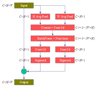
The experiments are based on the YOLOv5n model, as shown in Figure 3, the PR graphs of the YOLOv5n model for each category of images after improving the network structure, where the horizontal coordinate is the recall rate and the vertical coordinate is the precision rate, and the average recall-precision rate for each scene recognized using YOLOv5n is 0.7504.
The dataset used in the experiment is a small-scale screw and nut dataset, only two kinds of target (screw and nut) information are labeled in the dataset, and the labeling information includes target type and location information. There are 1700 sample pictures and 10963 labeled information in the dataset, and the maximum number of targets in each picture is 20 and the minimum is 3. During the experiment, 76.47% (1300) images in the dataset are randomly selected as training set samples, and the remaining 23.53% (400) images are used as test set samples.
Due to the small sample size, data enhancement is performed on the images during the test. Each time after reading the images from the training set, the images are randomly flipped, rotated, cropped, masked, hue transformed, brightness transformed and other operations are performed. The data enhancement randomly determines whether each transformation is executed and the magnitude of each transformation, which is equivalent to expanding the original small-scale dataset, and can effectively inhibit the degree of overfitting of the model and improve the final detection effect.
The experimental framework used is pytorch, and the operating system is Ubuntu18.04.4 LTS. The original YOLOv5 algorithm and the improved YOLOv5 algorithm are tested at the same time. The batch size, back propagation algorithm, learning rate, dataset, hardware and software environment and other settings are the same in the comparison test, except for the different network structures. The comparison of the loss value convergence curves of the two algorithms during training is shown in Figure 4, Fig. 4a shows YOLOv5 and Figure 4b shows the improved YOLOv5.
As can be seen in Figure 4, the improved YOLOv5 algorithm converges a little faster than the original YOLOv5 algorithm, with the YOLOv5 algorithm converging at 93 rounds and the improved YOLOv5 algorithm converging at 83 rounds. Due to the reduction in the number of model layers and the amount of parameters, the actual training time used is also much lower, YOLOv5 algorithm takes 30min to train 100 rounds, while the improved YOLOv5 algorithm takes only 20min.
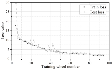
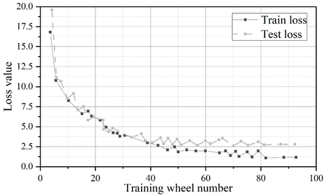
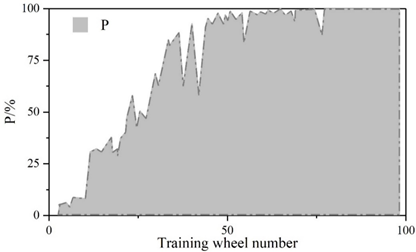
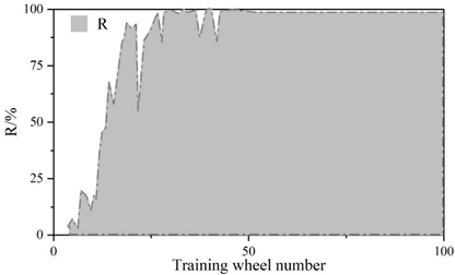
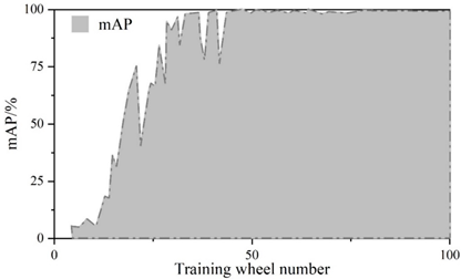
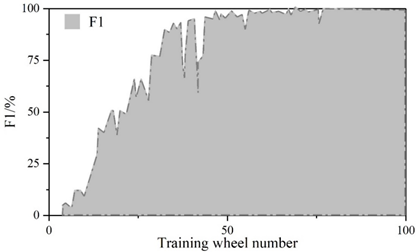
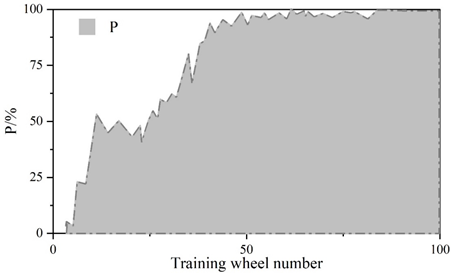
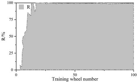
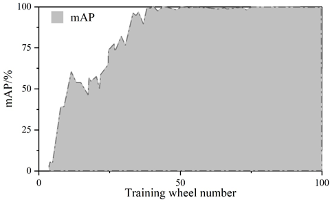
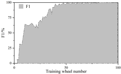
Figure 5 and Figure 6 show the convergence curves of the evaluation metrics of YOLOv5 algorithm and improved YOLOv5 algorithm, respectively.The experiment compares the change curves of the evaluation metrics of the two models during the training process.Similar to the loss values, the P, R, mAP, and F1 metrics reach the convergence position faster on the improved model.The values of the P, R, mAP, and F1 metrics of the YOLOv5 are 98.5%, 98.5%, 97.2%, 97.2%, 96.8%, and 96.8% respectively, 97%, 97.2%, and 97.8% for the improved YOLOv5 and 97%, 97%, 97%, and 96.8% for the metrics. The detection speeds of both were 42.6\(piece\bullet s^{-1}\) and 112.3\(piece\bullet s^{-1}\), respectively.
The scores of the indicators in the figure range from 0 to 1. The precision rate P of the improved YOLOv5 algorithm decreases by 1.5%, the recall rate R is the same, and the m AP decreases by 0.2% and the F1 value decreases by 1% in the comprehensive evaluation indicators. The larger the precision rate P and recall rate R indicates the better detection effect, but for the same algorithm P and R are negatively correlated, therefore, the m AP and F1 values of the comprehensive P and R indicators are generally used to measure the results. Test results show that: improved YOLOv5 algorithm in the detection of YOLOv5 algorithm has a substantial increase from an average of 42.6 sheets / s to 112.3 sheets / s, the detection speed about the effect of the original YOLOv5 algorithm compared with the original YOLOv5 algorithm is slightly reduced, but the gap is very small. The improvement in detection speed is 2.636 times that of the original algorithm, indicating that the Improved YOLOv5 algorithm performs better in terms of speed on this task dataset.
The improved YOLO v5 algorithm is able to accurately detect the location and type of all targets in the graph, and the difference between the predicted frame given by the algorithm and the actual ideal border is very small, which indicates that the improved YOLO v5 algorithm has better actual detection results.
In this paper, based on the deep convolutional neural network structure, YOLOv5 framework is introduced to construct the target detection algorithm. And in the YOLOv5 network model, a typical attention mechanism is incorporated to propose improvements to YOLOv5. At the same time, the loss function is added to realize the full convolutional network. Based on the evaluation index of the model, the target detection efficiency of the model is evaluated.
1) The improved YOLOV5n model is 2.9979 percentage points higher in MAP value than the original YOLOv5 model, and about 5.6211 and 7.9613 percentage points higher than the YOLOv7 and YOLOX effects, respectively.
2) The effectiveness of each part of the improvement is further verified by ablation experiments, where YOLOv5n_gcc has the same computational amount, the FPS decreases by 1, and the model accuracy improves from 85.564% to 86.354% compared with YOLOv5n_gc. At the same time, CIoU increases the detection capability of the model with a slight loss of detection time. The fully improved YOLOv5n_gcc improves the FPS substantially by 31% compared to YOLOv5n.
3) In the loss value and accuracy comparison, the improved YOLOv5 algorithm starts to converge at 83 rounds, and the time used for actual training is only 20 min, which saves 10 min compared to the original algorithm.