Counting nodes in Smolyak grids

1. Introduction

The aim of this article is to fill a gap in the literature by presenting a general framework which allows to produce explicit formulas for the number of nodes in a Smolyak grid.

Let $U_i$ be a quadrature rule on $[-1,1]$, i.e. $U_i:C^0([-1,1])\to \mathbb{R}$ or an interpolation rule i.e. $U_i:C^0([-1,1])\to C^0([-1,1])$ which evaluates an unknown function $g:[-1,1]\to \mathbb{R}$ on a finite set $S_i\subset [-1,1]$. The Smolyak rule turns a sequence of univariate quadrature or interpolation rules $U_1,U_2,\dots$ into a quadrature or interpolation rule on $[-1,1{]}^d$. Here, $|S_i|⩽|S_{i+1}|$ for all $i\in {\mathbb{N}}_{⩾1}$ and the Smolyak rule in $d$ dimensions of level $\mu \in \mathbb{N}$ is defined as $$\begin{array}{}\text{(1)}& Q_{\mu }^d=\sum _{d⩽|\mathbf{i}|⩽d+\mu }\underset{k=1}{\overset{d}{⨂}}{\mathrm{\Delta }}_{i_k},\end{array}$$ where ${\mathrm{\Delta }}_i=U_i-U_{i-1}$ as long as $i>2$ and ${\mathrm{\Delta }}_1=U_1$, $\mathbf{i}\in {\mathbb{N}}_{⩾1}^d$ is a multi-index with positive entries and $|\mathbf{i}|:=i_1+\dots +i_d$ denotes its $1$-norm (see [10]). [5] shows that (1) includes a lot of cancellation and can be expressed as (see also [11], Lemma 1).

$$Q_{\mu }^d=\sum _{max\{d,\mu +1\}⩽|\mathbf{i}|⩽d+\mu }(-1{)}^{d+\mu -|\mathbf{i}|}(\genfrac{}{}{0ex}{}{d-1}{d+\mu -|\mathbf{i}|})\underset{k=1}{\overset{d}{⨂}}{U}_{i_k}.$$

This last expression implies in which nodes an unknown function $u:[-1,1{]}^d\to \mathbb{R}$ needs to be evaluated, if $Q_{\mu }^d(u)$ is computed: We attach to the sequence $U_1,U_2,\dots$ of univariate quadrature or interpolation rules the sequence $\mathcal{S}=S_1,S_2,\dots$ of sets $S_i\subset [-1,1]$ of evaluation nodes such that $f(i)=|S_i|$ is a non-decreasing function $f:{\mathbb{N}}_{⩾1}\to {\mathbb{N}}_{⩾1}$, called growth function of $\mathcal{S}$. The Smolyak grid in $d$ dimensions with level $\mu$ is then given by $${\mathrm{\Gamma }}_d(\mu )=\bigcup _{max\{d,\mu +1\}⩽|\mathbf{i}|⩽d+\mu }{\times }_{k=1}^d{S}_{i_k}.$$

If the sequence $\mathcal{S}$ is nested, i.e. if $S_k\subset S_{k+1}$ for all $k\in {\mathbb{N}}_{⩾1}$, then $${\mathrm{\Gamma }}_d(\mu )=\bigcup _{|\mathbf{i}|=d+\mu }{\times }_{k=1}^d{S}_{i_k}.$$

Since the Smolyak rule has been introduced to overcome the curse of dimensionality, there is great interest in determining its computational cost i.e. to count the number of nodes in such a grid for a given sequence $\mathcal{S}$, a given dimension $d$ and a level $\mu$. This number will be denoted by ${\mathrm{N}}_d(\mu )$, where the growth function $f$ of the sequence $\mathcal{S}$ will be clear from the context. For our purposes, we consider isotropic grids but we remark that our counting argument at no point needs spatial isotropy but only that the sets used in each dimension share the same growth function.

For practical implementation, it might be of interest to count the number of nodes needed during the generating process of such grids, before duplicates are deleted, i.e. there might be interest in finding a simpler formula for $${\mathcal{N}}_d^{\mathrm{\Sigma }}(\mu )=\sum _{max\{d,\mu +1\}⩽|\mathbf{i}|⩽d+\mu }\prod _{k=1}^{d}f(i_k),$$ which doesn’t require to compute all the multi-indices $\mathbf{i}\in {\mathbb{N}}_{⩾1}^d$ such that $max\{d,\mu +1\}⩽|\mathbf{i}|⩽d+\mu$. The number ${\mathcal{N}}_d^{\mathrm{\Sigma }}(\mu )$ is of course independent of the nestedness or non-nestedness of the sequence $\mathcal{S}$, however, if the sequence is nested, counting points in the Smolyak grid with duplicates boils down to finding a formula for $${\mathcal{N}}_d(\mu )=\sum _{|\mathbf{i}|=d+\mu }\prod _{k=1}^{d}f(i_k).$$

We will provide formulas for the quantities ${\mathrm{N}}_d(\mu )$ for the case of $\mathcal{S}$ being nested and ${\mathcal{N}}_d(\mu )$ for general $\mathcal{S}$ only as $${\mathcal{N}}_d^{\mathrm{\Sigma }}(\mu )=\sum _{k=max\{0,\mu +1-d\}}^{\mu }{\mathcal{N}}_d(k).$$

For some specific growth functions, there are explicit formulas for ${\mathrm{N}}_d(\mu )$ available in the literature, see for instance [5,9, 2]. Also, a lot is known about upper bounds for ${\mathrm{N}}_d(\mu )$ or asymptotic formulas [9,5, 12,7, 11,8]. The contribution of [3] provides tables with values for ${\mathrm{N}}_d(\mu )$ and code which allows to generate them. Also, in [4], tables with values are provided.

Our approach allows to find closed formulas for the quantities ${\mathrm{N}}_d(\mu )$ and ${\mathcal{N}}_d(\mu )$ by using generating functions and dimension-wise induction, thus generalizing previous formulas obtained by of [8,7, 2] and [9]. To this end, we define $$G_d(x)=\sum _{\mu =0}^{\mathrm{\infty }}{\mathrm{N}}_d(\mu )x^{\mu }\text{ and }{\mathcal{G}}_d(x)=\sum _{\mu =0}^{\mathrm{\infty }}{\mathcal{N}}_d(\mu )x^{\mu }.$$

We are now ready to state our main result which will be restated for the convenience of the reader in Propositions 2.1 and 2.2:

We will include explicit formulas for some specific growth functions $f$ related to usual sequences $\mathcal{S}$ which are used in practice. Such sequences are for example based on:

1. Equidistant nodes without boundary: $$\mathring{\mathrm{E}}(n)=\{\frac{2k}{n+1}-1|k\in \{1,\dots ,n\}\},n\in {\mathbb{N}}_{⩾1}.$$

For these points, the sequence given by $S_k=\mathring{\mathrm{E}}(f(k))$ is nested if $f(k)=m^k-1$ for $m\in {\mathbb{N}}_{⩾2}$.

2. Equidistant nodes with boundary and Chebyshev nodes of the second kind: $$\mathrm{E}(n)=\{\frac{2(k-1)}{n-1}-1|k\in \{1,\dots ,n\}\},n\in {\mathbb{N}}_{⩾2},$$ $${\mathrm{C}}_2(n)=\{\cos \left(\frac{k-1}{n-1}\pi \right)|k\in \{1,\dots ,n\}\},n\in {\mathbb{N}}_{⩾2}.$$

The sequences $S_k=\mathrm{E}(f(k))$ and $S_k={\mathrm{C}}_2(f(k))$ respectively become nested if $f(k)=m^k+1$, $m\in {\mathbb{N}}_{⩾2}$. Sometimes it is convenient to define $\mathrm{E}(1)={\mathrm{C}}_2(1)=\{0\}$.

3. Chebyshev nodes of the first kind:

$${\mathrm{C}}_1(n)=\{\cos \left(\frac{2k-1}{2n}\pi \right)|k\in \{1,\dots ,n\}\},n\in {\mathbb{N}}_{⩾1}.$$

Here, the sequence $S_k={\mathrm{C}}_1(f(k))$ is nested if $f(k)=3^k$ or $f(k)=3^{k-1}$.

4. Leja nodes (see [6]): Any sequence $(x_n{)}_{n\in {\mathbb{N}}_{⩾1}}$ such that $x_1\in [-1,1]$ and $$x_n\in \underset{x\in [-1,1]}{\mathrm{a}\mathrm{r}\mathrm{g}\mathrm{m}\mathrm{a}\mathrm{x}}\prod _{j=1}^{n-1}|x-x_j|,n>1,$$ is called a Leja-sequence. For such a sequence, we let $$\mathrm{L}(n)=\{x_k|k\in \{1,\dots ,n\}\}.$$

Note that $S_k=\mathrm{L}(f(k))$ is nested for every choice of a non-decreasing growth function $f$, in particular, for $f(k)=k$. There is a symmetrized version of Leja nodes available which become nested for the growth function $f(k)=2k-1$ (see [1]).

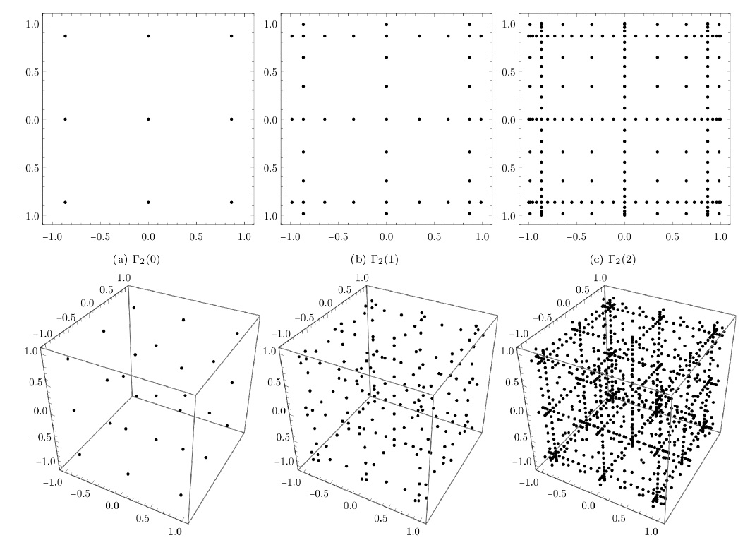
Example 1.2. Consider a Smolyak grid based on the sequence $\mathcal{S}$, where $S_k={\mathrm{C}}_1(3^k)$. As we show below, according to (3), one obtains $$\begin{array}{rl}{\mathrm{N}}_2(\mu )& =3^{\mu +1}(2\mu +3),\\ {\mathrm{N}}_3(\mu )& =3^{\mu +1}(2{\mu }^2+10\mu +9),\end{array}$$ so that the cardinalities in Figure 1 can be computed.

2. Counting nodes

We first consider a nested sequence $\mathcal{S}$ with growth function $f(k)=|S_k|$. Then we have the following proposition:

Let now $\mathcal{S}$ be a (not necessarily nested) sequence with growth function $f$ and consider the generating function $${\mathcal{G}}_d(x)=\sum _{\mu =0}^{\mathrm{\infty }}{\mathcal{N}}_d(\mu )x^{\mu }.$$

When discussing the applications of our main result, we will focus on nested sequences $\mathcal{S}$ but note that the formulas ${\mathcal{N}}_d(\mu )$ and ${\mathcal{N}}_d^{\mathrm{\Sigma }}(\mu )$ do not depend on the nestedness or non-nestedness of $\mathcal{S}$. The general recipe for obtaining an expression for ${\mathrm{N}}_d(\mu )$ or ${\mathcal{N}}_d(\mu )$ consists in evaluating $G_d$ and ${\mathcal{G}}_d$ respectively and then – for the growth functions under consideration – one can use Newton’s binomial theorem and the Cauchy product in order read off ${\mathrm{N}}_d(\mu )$ or ${\mathcal{N}}_d(\mu )$. We will provide the details for the first three growth functions under consideration – the others being obtained similarly:

2.1. Growth Function $f(k)=n^k-1$

In this case, ${\displaystyle G_1(x)=\frac{n-1}{(1-x)(1-nx)},}$ so that using Newton’s binomial theorem $$\begin{array}{rl}{G}_d(x)& =(n-1{)}^d{\left(\frac{1}{1-nx}\right)}^d\frac{1}{1-x},\\ & =(n-1{)}^d(\sum _{k=0}^{\mathrm{\infty }}(\genfrac{}{}{0ex}{}{d+k-1}{k})(nx{)}^k)\left(\sum _{\ell =0}^{\mathrm{\infty }}{x}^{\ell }\right).\end{array}$$

Reading off the coefficient of $x^{\mu }$ using the Cauchy product yields $${\mathrm{N}}_d(\mu )=(n-1{)}^d\sum _{k=0}^{\mu }(\genfrac{}{}{0ex}{}{d+k-1}{k})n^k.$$

Smiliarly we obtain $$\begin{array}{rl}{\mathcal{G}}_d(x)& =(n-1{)}^d{\left(\frac{1}{1-x}\right)}^d{\left(\frac{1}{1-nx}\right)}^d,\\ & =(n-1{)}^d(\sum _{k=0}^{\mathrm{\infty }}(\genfrac{}{}{0ex}{}{d+k-1}{k})(nx{)}^k)\left(\sum _{\ell =0}^{\mathrm{\infty }}(\genfrac{}{}{0ex}{}{d+\ell -1}{\ell })x^{\ell }\right).\end{array}$$

The coefficient of the term $x^{\mu }$ is therefore $${\mathcal{N}}_d(\mu )=(n-1{)}^d\sum _{k=0}^{\mu }(\genfrac{}{}{0ex}{}{d+k-1}{k})(\genfrac{}{}{0ex}{}{d+\mu -k-1}{\mu -k})n^k.$$

2.2. Growth function $f(k)=n^k$

Here, ${\displaystyle G_1(x)=\frac{n}{1-nx},}$ so that $$\begin{array}{rl}{G}_d(x)& =n^d{\left(\frac{1}{1-nx}\right)}^d(1-x{)}^{d-1},\\ & =n^d(\sum _{k=0}^{d-1}(\genfrac{}{}{0ex}{}{d-1}{k})(-1{)}^k{x}^k)(\sum _{\ell =0}^{\mathrm{\infty }}(\genfrac{}{}{0ex}{}{d+\ell -1}{\ell })(nx{)}^{\ell }).\end{array}$$

Reading off the coefficient of $x^{\mu }$ leads to $$\begin{array}{}\text{(3)}& {\mathrm{N}}_d(\mu )=n^d\sum _{k=0}^{min\{d-1,\mu \}}(\genfrac{}{}{0ex}{}{d-1}{k})(-1{)}^k(\genfrac{}{}{0ex}{}{d+\mu -k-1}{\mu -k})n^{\mu -k},\end{array}$$ which can be shown to be equivalent to $$\begin{array}{}\text{(4)}& {\mathrm{N}}_d(\mu )=\sum _{k=0}^{min\{d-1,\mu \}}(\genfrac{}{}{0ex}{}{d-1}{k})(\genfrac{}{}{0ex}{}{\mu }{k})n^{\mu +d-k}(n-1{)}^k.\end{array}$$

Similarly, $${\mathcal{G}}_d(x)=n^d{\left(\frac{1}{1-nx}\right)}^d=n^d(\sum _{k=0}^{\mathrm{\infty }}(\genfrac{}{}{0ex}{}{d+k-1}{k})(nx{)}^k),$$ so that the coefficient of $x^{\mu }$ can be read off and one obtains $${\mathcal{N}}_d(\mu )=n^{d+\mu }(\genfrac{}{}{0ex}{}{d+\mu -1}{\mu }).$$

2.3. Growth function $f(k)=n^k+1$

Here, $$\begin{array}{rl}{G}_1(x)=& \frac{n+1-2nx}{(1-x)(1-nx)},\\ {\mathrm{N}}_d(\mu )=& \sum _{k=0}^{min\{d,\mu \}}(\genfrac{}{}{0ex}{}{d}{k})(-2n{)}^k(n+1{)}^{d-k}\sum _{\ell =0}^{\mu -k}(\genfrac{}{}{0ex}{}{d+\ell -1}{\ell })n^{\ell }.\end{array}$$

Furthermore, in this case, ${\displaystyle {\mathcal{G}}_d(x)=(n+1-2nx{)}^d{\left(\frac{1}{1-nx}\right)}^d{\left(\frac{1}{1-x}\right)}^d,}$ so that

$${\mathcal{N}}_d(\mu )=\sum _{\ell =0}^{min\{d,\mu \}}\sum _{k=0}^{\mu -\ell }(\genfrac{}{}{0ex}{}{d}{\ell })(-1{)}^{\ell }(2n{)}^{\ell }(n+1{)}^{d-\ell }(\genfrac{}{}{0ex}{}{d+k-1}{k})(\genfrac{}{}{0ex}{}{d+\mu -\ell -k-1}{\mu -\ell -k})n^k.$$

2.4. Growth function $f(k)=k$

Here, $G_1(x)=\frac{1}{(1-x{)}^2}$ so that ${\displaystyle G_d(x)=\frac{1}{(1-x{)}^{d+1}}=\sum _{k=0}^{\mathrm{\infty }}(\genfrac{}{}{0ex}{}{d+k}{k})x^k,}$ and hence $${\mathrm{N}}_d(\mu )=(\genfrac{}{}{0ex}{}{d+\mu }{\mu }).$$

Similarly, we obtain $${\mathcal{G}}_d(x)=\frac{1}{(1-x{)}^{2d}}=\sum _{k=0}^{\mathrm{\infty }}(\genfrac{}{}{0ex}{}{2d+k-1}{k})x^k,$$ and hence $${\mathcal{N}}_d(\mu )=(\genfrac{}{}{0ex}{}{2d+\mu -1}{\mu }).$$

In this case, we obtain setting $m=max\{0,\mu +1-d\}$: $${\mathcal{N}}_d^{\mathrm{\Sigma }}(\mu )=\frac{1}{2d}((1+\mu )(\genfrac{}{}{0ex}{}{2d+\mu }{\mu +1})-m(\genfrac{}{}{0ex}{}{2d+m-1}{m})).$$

2.5. Further remarks

If $f(k)=2^{k-1}+1$ for $k>1$ and $f(1)=1$, one can show by induction on $d$ using (2) that ${\mathrm{N}}_d(\mu )-1=2^{\mu }{P}_{d-1}(\mu ),$ where $P_{d-1}$ is a polynomial of degree $d-1$ with leading coefficient $1/(2^{d-1}(d-1)!)$ so that one obtains the asymptotics $${\mathrm{N}}_d(\mu )\sim \frac{2^{\mu }}{2^{d-1}(d-1)!}{\mu }^{d-1},$$ for $d$ fixed and $\mu \to \mathrm{\infty }$, compare [7, Lemma 1].

Using $f(k)=2k-1$ yields ${\displaystyle G_1(x)=\frac{1+x}{(1-x{)}^2},}$ so that ${\displaystyle G_d(x)=\frac{(1+x{)}^d}{(1-x{)}^{d+1}},}$ and hence $${\mathrm{N}}_d(\mu )=\sum _{k=0}^{min\{d,\mu \}}(\genfrac{}{}{0ex}{}{\mu }{k})(\genfrac{}{}{0ex}{}{\mu +d-k}{\mu }),$$ which is precisely Theorem 2 of [8]. We note that this formula is also obtained using generating functions.

Acknowledgments

This study has been financed by the “Ingénierie et Architecture” domain of HES-SO, University of Applied Sciences Western Switzerland, which is acknowledged. We further thank the referees for their careful reading and their valuable comments and suggestions.