
An open-locating-dominating set can model a type of detection system which determines the location of a possible “intruder” for a facility or a possible faulty processor in a network of processors [13]. A detection system is an extensively studied graphical concept which is also known as a watching system or discriminating codes [1, 2]. Various detection systems have been defined based on the functionality of each detector in the system. Other well-known and much studied detection systems include identifying codes [9], locating-dominating sets [15] (See Lobstein’s Bibliography [7] for a list of the articles in this field.). In this paper, we consider a fault-tolerant variant of an open-locating dominating set called error-detecting open-locating-dominating sets. We present more results on the topic including its NP-completeness proof, extremal graphs, and a characterization in cubic graphs.
Let \(G\) be a graph with vertices \(V(G)\) and edges \(E(G)\). The open-neighborhood of a vertex \(v \in V(G)\), denoted \(N(v)\), is the set of all vertices adjacent to \(v\): \(\{w \in V(G) : vw \in E(G)\}\). The closed-neighborhood of a vertex \(v \in V(G)\), denoted \(N[v]\), is the set of all vertices adjacent to \(v\), as well as \(v\) itself: \(N(v) \cup \{v\}\). An open-dominating set (also called total-dominating) \(S\) of a graph \(G\) is a subset of vertices where every vertex has a neighbor in \(S\). An open-locating-dominating set (OLD set) \(S\) of a graph \(G\) is an open-dominating set such that each pair of distinct vertices in \(G\) have distinct open-neighborhoods within \(S\). For an OLD set \(S \subseteq V(G)\) and \(u \in V(G)\), we let \(N_S(u) = N(u) \cap S\) denote the dominators of \(u\) and \(dom(u) = |N_S(u)|\) denote the (open) domination number of \(u\). A vertex \(v \in V(G)\) is \(k\)-open-dominated by an open-dominating set \(S\) if \(|N_S(v)| = k\). If \(S\) is a open-dominating set and \(u,v \in V(G)\), \(u\) and \(v\) are \(k\)-distinguished if \(|N_S(u) \triangle N_S(v)| \ge k\), where \(\triangle\) denotes the symmetric difference. If \(S\) is a open-dominating set and \(u,v \in V(G)\), \(u\) and \(v\) are \(k^\#\)-distinguished if \(|N_S(u) – N_S(v)| \ge k\) or \(|N_S(v) – N_S(u)| \ge k\). We will also use terms such as “at least \(k\)-dominated” to denote \(j\)-dominated for some \(j \ge k\).
There are several fault-tolerant variants of OLD sets. For example, a redundant open-locating-dominating set is resilient to a detector being destroyed or going offline [14]. Thus, an open-dominating set \(S \subseteq V(G)\) is called a redundant open-locating-dominating (RED:OLD) set if \(\forall v \in S\), \(S – \{v\}\) is an OLD set. The focus of this paper is another variant of an OLD set called an error-detecting open-locating-dominating (DET:OLD) set, which is capable of correctly identifying an intruder even when at most one sensor or detector incorrectly reports that there is no intruder. Hence, DET:OLD sets allow for uniquely locating an intruder in a way which is resilient to up to one false negative. The following Theorem characterizes OLD, RED:OLD, and DET:OLD sets and they are useful in constructing those sets or verifying whether a given set meets their requirements.
Theorem 1.1. An open-dominating set is
i. an OLD set if and only if every pair of vertices is 1-distinguished [8].
ii. a RED:OLD set if and only if all vertices are at least 2-dominated and all pairs are 2-distinguished [14].
iii. a DET:OLD set if and only if all vertices are at least 2-dominated and all pairs are \(2^\#{}\)-distinguished [14].
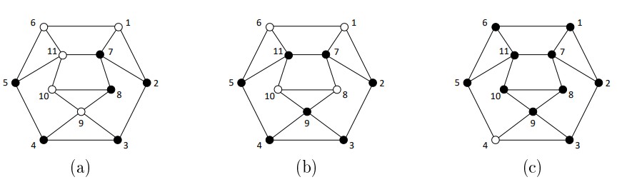
Figure 1 shows OLD, RED:OLD, and DET:OLD sets on the given graph \(G\); we can verify exhaustively that these sets of detectors meet the requirements of Theorem 1.1. To understand why the conditions of DET:OLD established in Theorem 1.1 are necessary, consider the following example scenarios. Suppose we use the RED:OLD detector set from Figure 1 (b) and there is an in intruder at \(v_9\); then precisely two vertices, \(v_3\) and \(v_4\), will detect the intruder. However, if \(v_3\) gives a false negative, we will have only \(v_4\) detecting an intruder. This detection pattern is identical to an alternative scenario where the intruder is placed at \(v_5\) and \(v_{11}\) gives a false negative response. Because there are two scenarios in which we observe the same detection pattern for two different intruder locations (\(v_5\) and \(v_9\)), we fail to locate the intruder; in particular, we find that \(v_5\) and \(v_9\) are 2-distinguished but not \(2^{\#}\)-distinguished. However, if we reattempt the same scenario using instead the detector set from Figure 1 (c), we see that the intruder at \(v_9\) causes detections at \(v_3\), \(v_8\), and \(v_{10}\). Suppose one of these three detectors reports a false negative; for the sake of example let \(v_{10}\) give a false negative. We still have two positive responses from \(v_3\) and \(v_8\), so the intruder must be within \(N(v_3) \cap N(v_8)\), which contains only \(v_9\); thus, we have successfully located the intruder despite the false negative. From Theorem 1.1, we see that the only difference between RED:OLD and DET:OLD is the switch from 2-distinguishing in RED:OLD to the stronger \(2^{\#}\)-distinguishing in DET:OLD. It is ultimately this additional requirement of \(2^{\#}\)-distinguishing that allows DET:OLD to overcome the possibility of false negatives and still locate intruders; the full proof of this fact is available in [14].
Naturally, our goal is to install a minimum number of detectors in any detection system. For finite graphs, the notations \(\textrm{OLD}(G)\), \(\textrm{RED:OLD}(G)\), and \(\textrm{DET:OLD}(G)\) represent the cardinality of the smallest possible OLD, RED:OLD, and DET:OLD sets on graph \(G\), respectively [8, 12, 14]. We can verify exhaustively that the sets presented in Figure 1 are optimal, as there are no smaller sets meeting their respective requirements on this graph. Therefore, we have \(\textrm{OLD}(G) = 6\), \(\textrm{RED:OLD}(G) = 7\), and \(\textrm{DET:OLD}(G) = 10\).
When measuring detector sets on infinite graphs, instead of cardinality, we use the density of the subset, which is conceptually the ratio of the number of detectors to the total number of vertices. Formally, the density of \(S \subseteq V(G)\) is defined as \(\limsup_{r \to \infty}\frac{|B_r(x) \cap S|}{|B_r(x)|}\), where \(B_r(v) = \{u \in V(G) : d(u,v) \le r\}\) is the ball of radius \(r\) about \(v\) and \(x\) is a particular choice of center point for the expansion. Notably, this definition of density is a function of the center vertex, \(x\); however, it has been proven that graphs exhibiting the “slow-growth” property of \(\lim_{r \to \infty}\frac{|B_{r+1}(x)|}{|B_r(x)|} = 1\) for some choice of \(x \in V(G)\) have the additional property that the density is invariant of the chosen center point [10]. In this paper, we will only consider graphs which exhibit this slow-growth property. With the formal definition of density established for both finite and infinite graphs, the notations \(\textrm{OLD}%(G)\), \(\textrm{RED:OLD}%(G)\), and \(\textrm{DET:OLD}%(G)\) represent the minimum density of such a set on \(G\).
In Section 2, we present extremal graphs with the highest value of \(\textrm{DET:OLD%}(G)\). In Section 3, we provide a proof that the problem of determining \(\textrm{DET:OLD}(G)\) for an arbitrary graph is NP-complete. Sections 4 and 5 discuss DET:OLD sets on several infinite grids and cubic graphs, respectively.
In this section, we consider extremal graphs with \(\textrm{DET:OLD}(G) = n\). Let \(S \subseteq V(G)\) be a DET:OLD set for \(G\); because non-detectors do not aid in locating intruders, it must be that \(S\) is a DET:OLD set for \(G – (V(G) – S)\), implying the smallest graph with DET:OLD will have \(\textrm{DET:OLD}(G) = n\). The following theorem shows that the smallest graphs with DET:OLD have \(n = 7\).
Theorem 2.1. If \(G\) has a DET:OLD, then \(n \ge 7\).
Proof. Assume to the contrary, \(n \le 6\). Clearly \(G\) has a cycle because DET:OLD requires \(\delta(G) \ge 2\). Firstly, we consider the cases when the smallest cycle in the graph is \(C_n\), with n = 6,5,4. If the smallest cycle is a \(C_6\) subgraph \(abcdef\), then \(a\) and \(c\) cannot be distinguished without having \(n \ge 7\), a contradiction. Suppose the smallest cycle is a \(C_5\) subgraph \(abcde\). To distinguish \(a\) and \(c\), by symmetry we can assume that \(\exists u \in N(a) – N(c) – \{a,b,c,d,e\}\). Similarly, to distinguish \(b\) and \(e\) we can assume by symmetry that \(\exists v \in N(b) – N(e) – \{a,b,c,d,e\}\). If \(u = v\), there would be a smaller cycle, implying \(n \ge 7\), a contradiction; thus, we can assume \(u \neq v\). Suppose the smallest cycle is a \(C_4\) subgraph \(abcd\). To distinguish \(a\) and \(c\), we can assume \(p,q \in N(a) – N(c) – \{a,b,c,d\}\). Similarly, to distinguish \(b\) and \(d\) we can assume by symmetry that \(\exists x,y \in N(b) – N(d) – \{a,b,c,d\}\). We know that \(\{p,q\} \cap \{x,y\} = \varnothing\) because otherwise we create a smaller cycle; thus, \(n \ge 8\), a contradiction. Otherwise, we can assume that \(G\) has a triangle.
Next, we will show that if \(G\) contains a \(K_4\) subgraph, then \(n \ge 7\); let \(abcd\) be the vertices of a \(K_4\) subgraph in \(G\). To distinguish pairs of vertices in \(abcd\), without loss of generality we can assume that \(\exists x \in N(a)\), \(\exists y \in N(b)\), and \(\exists z \in N(c)\). Clearly \(\{x,y,z\} \cap \{a,b,c,d\} = \varnothing\) because \(x\), \(y\), and \(z\) are used to distinguish the vertices \(a\), \(b\), \(c\), and \(d\); however, we do not yet know if \(x\), \(y\), and \(z\) are distinct. If \(x=y=z\), then distinguishing \(a\), \(b\), and \(c\) requires at least another two vertices, so we would have at least 7 vertices and would be done; otherwise, without loss of generality we can assume \(x \neq z\). Suppose \(x=y\); we see that \(a\) and \(b\) are not distinguished and \(n=6\), so without loss of generality let \(bz \in E(G)\) to distinguish \(a\) and \(b\). If \(\{dx,dz\} \cap E(G) = \varnothing\), then \((d,x)\) and \((d,z)\) cannot be distinguished; otherwise without loss of generality assume \(dx \in E(G)\). We now see that \(a\) and \(d\) are not distinguished, but they are symmetric, so without loss of generality let \(dz \in E(G)\) to distinguish \(a\) and \(d\). We see that \(d\) and \(b\) become closed twins and cannot be distinguished. Otherwise, we can assume \(x \neq y\) and by symmetry \(y \neq z\). Thus, \(n \ge 7\), and we would be done. Thus, if \(G\) has a \(K_4\) subgraph, then we would be done.
Next, we will show that the existence of a “diamond” subgraph, which is an (almost) \(K_4\) subgraph minus one edge, implies that \(n \ge 7\). Let \(abcd\) be a \(C_4\) subgraph and assume \(ac \in E(G)\) but \(bd \notin E(G)\), which forms said diamond subgraph. To distinguish \(b\) and \(d\), we can assume by symmetry that \(\exists u,v \in N(b) – N(d) – \{a,b,c,d\}\). Similarly, to distinguish \(a\) and \(c\), we can assume that \(\exists w \in N(a) – N(c) – \{a,b,c,d\}\). We know that \(u \neq v\) by assumption, so \(n \le 6\) requires by symmetry that \(w = u\). We can assume that \(uc \notin E(G)\) because otherwise this would create a \(K_4\) subgraph and fall into a previous case. We see that \(cv \in E(G)\) is required to distinguish \(u\) and \(c\). To distinguish \(u\) and \(v\), by symmetry we can assume \(uv \in E(G)\). Now, we see that \(a\) and \(v\) cannot be distinguished without creating a \(K_4\) subgraph, so we are done with the diamond case.
For the final case, we know there must be a triangle, \(abc\), but there cannot be any \(K_4\) or diamond subgraphs. To distinguish vertices in \(abc\), we can assume by symmetry that \(\exists u \in N(a) – \{a,b,c\}\) and \(\exists v \in N(b) – \{a,b,c\}\); further, we know that \(u \neq v\) because otherwise this would create a diamond subgraph. We know that \(\{av, bu, cu, cv\} \cap E(G) = \varnothing\) because any of these edges would create a diamond subgraph. Suppose \(uv \in E(G)\); then distinguishing \(a\) and \(v\) within the bounds of \(n \le 6\) requires \(\exists w \in N(a) – N(v) – \{a,b,c,u,v\}\). Similarly, distinguishing \(u\) and \(b\) requires \(w \in N(b)\); however, this creates a diamond subgraph, so we would be done. Otherwise, we can assume that \(uv \notin E(G)\). To 2-dominate \(u\) and \(v\), we require \(\exists p \in N(u) – \{a,b,c,u,v\}\) and \(\exists q \in N(v) – \{a,b,c,u,v\}\). However, \(n \le 6\) requires that \(p = q\). We see that \(u\) and \(v\) cannot be distinguished without creating a diamond subgraph or having \(n \ge 7\), completing the proof. ◻
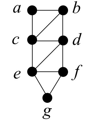
Let \(G_{n,m}\) have \(n\) vertices and \(m\) edges. Then \(G_{7,11}\), as shown in Figure 2, is the first graph that permits a DET:OLD set in the lexicographic ordering of \((n,m)\) tuples; i.e., the graph with the smallest number of edges given the smallest number of vertices.
Next we consider extremal graphs with \(\textrm{DET:OLD}(G) = n\) with the fewest number of edges.
Observation 2.2. If \(S\) is a DET:OLD set on \(G\) and \(v \in V(G)\), then \(v\) has at most one degree 2 neighbor.
Theorem 2.3. If \(G_{n,m}\) has DET:OLD then \(m \ge \left\lceil \frac{3n – \left\lfloor \frac{n}{2} \right\rfloor}{2} \right\rceil\).
Proof. Because \(G\) has DET:OLD, we know \(\delta(G) \ge 2\); let \(p\) be the number of degree 2 vertices in \(G\). By Observation 2.2, every degree 2 vertex, \(v\), must have at least one neighbor, \(u\), of at least degree 3, and said neighbor \(u\) is not adjacent to any degree 2 vertices other than \(v\). Thus, we can pair each of the \(p\) degree 2 vertices with a unique degree 3 or higher vertex. From this we know that \(p \le \left\lfloor \frac{n}{2} \right\rfloor\), and the \(n-2p\) vertices that are not pairs are all at least degree 3. Thus, \(\sum\limits_{v \in V(G)}{deg(v)} \ge (2 + 3)p + 3(n – 2p) = 3n – p \ge 3n – \left\lfloor \frac{n}{2} \right\rfloor\). However, we also know that the degree sum of any graph must be even, so we can strengthen this to \(\sum\limits_{v \in V(G)}{deg(v)} \ge 2 \left\lceil \frac{3n – \left\lfloor \frac{n}{2} \right\rfloor}{2} \right\rceil\). Dividing the degree sum by 2 completes the proof. ◻
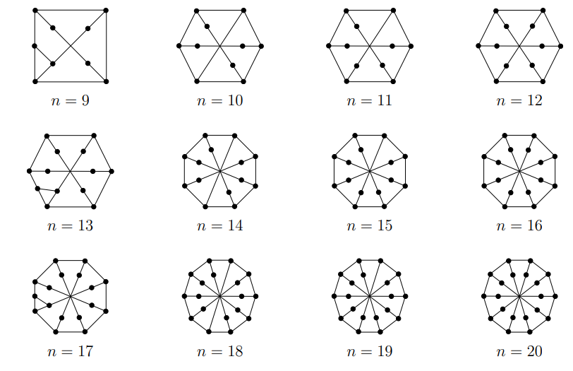
The lower bound given in Theorem 2.3 on the minimum number of edges in a graph with DET:OLD is sharp for all \(n \ge 9\) and Figure 3 shows a construction for an infinite family of graphs achieving the extremal value for \(9 \le n \le 20\).
It has been shown that finding the cardinality of the smallest OLD set, when phrased as a decision problem, is NP-complete [13]. This NP-completeness has also been demonstrated for many other forms of detection systems explored in other works, such as the Locating-Dominating set [5, 3] and the Identifying Code [3, 4]. We will now prove that the problem of determining the smallest DET:OLD set is also NP-complete. For additional information about NP-completeness, see Garey and Johnson [6].
Question 3.1(3-SAT).Let \(X\) be a set of \(N\) variables. Let \(\psi\) be a conjunction of \(M\) clauses, where each clause is a disjunction of three literals from distinct variables of \(X\). Is there is an assignment of values to \(X\) such that \(\psi\) is true?
Question 3.2(Error-Detecting Open-locating dominating set (DET-OLD)).A graph \(G\) and integer \(K\) with \(7 \le K \le |V(G)|\). Is there a DET:OLD set \(S\) with \(|S| \le K\)? Or equivalently, is \(\textrm{DET:OLD}(G) \le K\)?
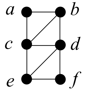
Lemma 3.3. In the \(G_6\) subgraph given in Figure 4, all six vertices internal to \(G_6\), as well as at least one external vertex adjacent to \(b\) must be detectors in order for DET:OLD to exist.
Proof. Note that vertices \(a\), \(b\), and \(d\) are permitted to have any number of edges going to vertices outside of the \(G_6\) subgraph under consideration, but no other edges incident with these 6 vertices are allowed. Suppose \(S\) is a DET:OLD for \(G\). Firstly, to 2-dominate \(f\), we require \(\{e,d\} \subseteq S\). To distinguish \(e\) and \(f\), we require \(\{c,f\} \subseteq S\). To distinguish \(c\) and \(f\), we require \(\{a,b\} \subseteq S\). Finally, \(e\) and \(b\) are not distinguished unless \(b\) is adjacent to at least one detector external to this \(G_6\) subgraph, completing the proof. ◻
Theorem 3.4. The DET-OLD problem is NP-complete.
Proof. Clearly, DET-OLD is NP, as every possible candidate solution can be generated nondeterministically in polynomial time (specifically, \(O(n)\) time), and each candidate can be verified in polynomial time using Theorem 1.1. To complete the proof, we will now show a reduction from 3-SAT to DET-OLD.
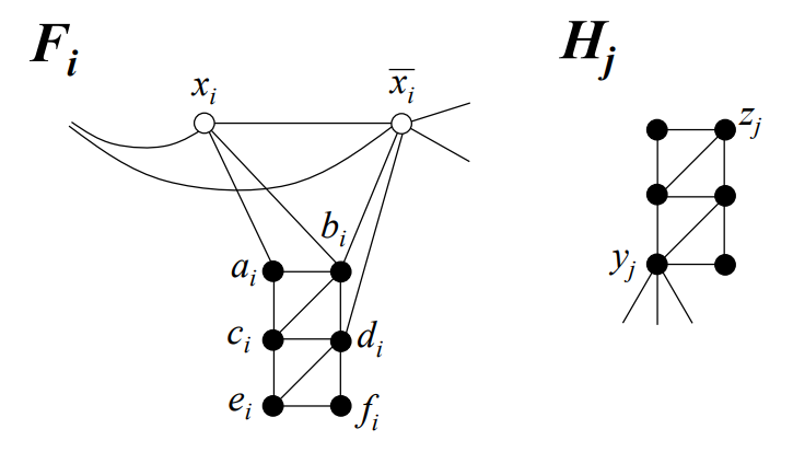
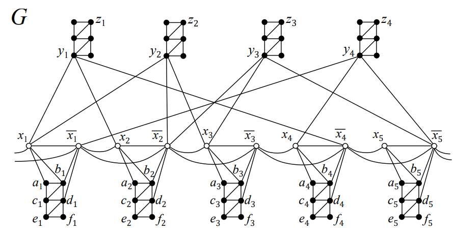
Let \(\psi\) be an instance of the 3-SAT problem with \(M\) clauses on \(N\) variables. We will construct a graph, \(G\), as follows. For each variable \(x_i\), create an instance of the \(F_i\) graph (Figure 5); this includes a vertex for \(x_i\) and its negation \(\overline{x_i}\). For each \(i \in \{1, …, N\}\), let \(\{\overline{x_i}\;\!x_k, \overline{x_i}\,\overline{x_k}\} \subseteq E(G)\) for \(k = (i \!\!\mod N) + 1\). For each clause \(c_j\) of \(\psi\), create a new instance of the \(H_j\) graph (Figure 5). For each clause \(c_j = \alpha \lor \beta \lor \gamma\), create an edge from the \(y_j\) vertex to \(\alpha\), \(\beta\), and \(\gamma\) from the variable graphs, each of which is either some \(x_i\) or \(\overline{x_i}\); for an example, see Figure 6. The resulting graph has precisely \(8N + 6M\) vertices and \(16N + 12M\) edges, and can be constructed in polynomial time. To complete the problem instance, we define \(K = 7N + 6M\).
Suppose \(S \subseteq V(G)\) is a DET:OLD on \(G\) with \(|S| \le K\). By Lemma 3.3, we require at least the \(6N + 6M\) detectors shown by the shaded vertices in Figure 5. Additionally, Lemma 3.3 gives us the additional requirement that each \(b_i\) vertex must be dominated by at least one additional detector outside of its \(G_6\) subgraph; thus, for each \(i\), \(\{x_i,\overline{x_i}\} \cap S \neq \varnothing\), giving us at least \(N\) additional detectors. Thus, we find that \(|S| \ge 7N + 6M = K\), implying that \(|S| = K\), so \(|\{x_i,\overline{x_i}\} \cap S| = 1\) for each \(i \in \{1, …, N \}\). Applying Lemma 3.3 again to the clause graphs yields that each \(y_j\) vertex must be dominated by at least one additional detector outside of its \(G_6\) subgraph. As no more detectors may be added, it must be that each \(y_j\) is now dominated by one of its three neighbors in the \(F_i\) graphs; therefore, \(\psi\) is satisfiable.
For the converse, suppose we have a solution to the 3-SAT problem \(\psi\); we will show that there is a DET:OLD, \(S\), on \(G\) with \(|S| \le K\). We construct \(S\) by first including all of the \(6N + 6M\) vertices as shown in Figure 5. Next, for each variable, \(x_i\), if \(x_i\) is true then we let the vertex \(x_i \in S\); otherwise, we let \(\overline{x_i} \in S\). Thus, the fully-constructed \(S\) has \(|S| = 7N + 6M = K\). Each \(b_i\) has its required external dominator due to having \(x_i \in S\) or \(\overline{x_i} \in S\). Additionally, because \(S\) was constructed from a satisfying truth assignment for the 3-SAT problem, by hypothesis each \(y_j\) vertex must also be dominated by one of its (external) term vertices in the \(F_i\) subgraphs. Therefore, each \(G_6\) subgraph in \(G\) satisfies Lemma 3.3, and so are internally sufficiently dominated and distinguished. Since all \(G_6\) subgraphs are sufficiently far apart, it is also the case that all vertex pairs in distinct \(G_6\) subgraphs are distinguished. Indeed, it can be shown that all vertices are 2-dominated and \(2^\#{}\)-distinguished, so \(S\) is a DET:OLD set for \(G\) with \(S \le K\), completing the proof. ◻
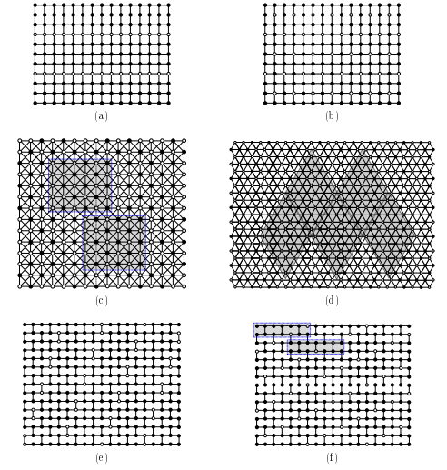
In this section we consider minimum-sized DET:OLD sets on the infinite hexagonal grid (HEX), the infinite square grid (SQR), the infinite triangular grid (TRI), and the infinite king grid (KNG). Figure 7 presents the best constructions that have been discovered so far. Solutions (b), (c), and (f) are new solutions, while the others were first presented in other papers [8, 14]. The solutions for HEX, SQR, and TRI are tight bounds, while the exact value for KNG is currently unknown. Subfigure (c) gives the best (i.e., lowest-density) solution we have constructed for KNG.
To establish lower bounds for the minimum densities of domination-based parameters in infinite graphs, we employ a concept known as a share argument, originally introduced by Slater [16] and extensively utilized by other literature [8, 11]. Essentially, this technique inverts the problem: instead of directly seeking a lower bound for the density of a DET:OLD set, we determine an upper bound on the average share of a detector vertex \(v \in S\), denoted \(sh(v) = \sum\limits_{u \in N(v)}{\frac{1}{dom(u)}}\), representing its total contribution to the domination of its neighbors. Because \(S\) is an open-dominating set, every vertex is at least 1-open-dominated, and each vertex with \(dom(u) = k\) contributes precisely \(\frac{1}{k}\) to the share of each of its \(k\) dominators, for a total of \(1\) per vertex in \(V(G)\). Therefore, an upper bound for the average share of all detectors can be inverted to yield a lower bound for the density of \(S\) in \(V(G)\).
As an example of how share could be used to produce a lower bound for \(\textrm{DET:OLD%}(G)\), suppose \(G\) is \(k\)-regular and let \(v \in S\) be an arbitrary detector vertex in some DET:OLD set \(S \subseteq V(G)\). We know that \(v\) has \(k\) neighbors and each neighbor must be at least 2-dominated due to \(S\) being a DET:OLD set. Therefore, \(sh(v) \le \frac{1}{2} + \frac{1}{2} + … + \frac{1}{2} + \frac{1}{2} = \frac{k}{2}\). Because \(v\) was selected arbitrarily, this value of \(\frac{k}{2}\) serves as an upper bound for the average share of all detectors, and so its inverse, \(\frac{2}{k}\), represents a lower bound for the minimum density of a DET:OLD set in \(G\). Because KNG is 8-regular, we get a trivial lower bound of \(\textrm{DET:OLD%}(\textrm{KNG}) \ge \frac{1}{4}\); next, we will present a proof for a better lower bound. In the proof, as a shorthand, we will let \(\sigma_A\) denote \(\sum\limits_{k \in A}{\frac{1}{k}}\) for some sequence of single-character symbols, \(A\). For example, \(\sigma_a = \frac{1}{a}\), \(\sigma_{ab} = \frac{1}{a} + \frac{1}{b}\), and so on.
Theorem 4.1. The infinite king grid, KNG, has \(\textrm{DET:OLD}%(\textrm{KNG}) \ge \frac{3}{8}\).
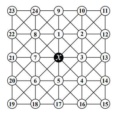
Proof. We will use the labeling shown in Figure 8. Let \(S \subseteq V(G)\) be a DET:OLD set and \(x \in S\). We will show that \(sh(x) \le \frac{8}{3}\), which would complete the proof. Firstly, we know that each vertex must be at least 2-dominated. If there are two distinct vertices \(p,q \in N(x)\) with \(dom(p) = dom(q) = 2\), then \(p\) and \(q\) cannot be distinguished; therefore, we may assume that there is at most one 2-dominated vertex in \(N(x)\). Suppose that \(dom(v_1) \le 3\) and \(dom(v_2) \le 3\) and \(dom(v_3) \le 3\). By inspecting \(v_1\) and \(v_2\), we see that if \((N_S(v_1) \cap N_S(v_2)) – \{x\} \neq \varnothing\), then \(v_1\) and \(v_2\) cannot be distinguished; thus, we can assume that \(\{v_3,v_9,v_{10}\} \cap S = \varnothing\). By applying this same logic to \(v_2\) and \(v_3\), we arrive at \(\{v_1,v_{12},v_{13}\} \cap S = \varnothing\). And by applying this logic a final time with \(v_1\) and \(v_3\), we have \(v_2 \notin S\). We see that vertex \(v_2\) can only be 2-dominated, so it must be the (only) 2-dominated vertex in \(N(x)\). Now suppose that \(dom(v_4) = dom(v_5) = 3\). By applying similar pairwise reasoning to vertices in \(\{v_3,v_4,v_5\}\), we find that \(dom(v_4) = 2\), a contradiction. Otherwise, we know that \(dom(v_4) \ge 4\) or \(dom(v_5) \ge 4\), and by symmetry we also have that \(dom(v_7) \ge 4\) or \(dom(v_8) \ge 4\). In any case, we see that \(sh(x) \le \sigma_{24433333} = \frac{1}{2} + \frac{2}{4} + \frac{5}{3} = \frac{8}{3}\), and we would be done. Otherwise, we know that vertices \(\{v_1,v_2,v_3\}\) must contain at least one vertex which is at least 4-dominated, and by symmetry for any \(A \in \{\{v_3,v_4,v_5\}, \{v_5,v_6,v_7\}, \{v_1,v_7,v_8\}\}\), \(A\) must contain at least one vertex which is at least 4-dominated. These four “corner” regions may be satisfied by as few as two 4-dominated vertices, resulting in \(sh(x) \le \sigma_{24433333} = \frac{8}{3}\) and completing the proof. ◻
The following theorem summarizes upper and lower bounds for DET:OLD on the four infinite grids we have explored.
Theorem 4.2. The upper and lower bounds on DET:OLD:
i. For the infinite hexagonal grid HEX, \(\textrm{DET:OLD%}(HEX) = \frac{6}{7}\). (Seo and Slater [14])
ii. For the infinite square grid SQR, \(\textrm{DET:OLD%}(SQR) = \frac{3}{4}\). (Seo and Slater [14])
iii. For the infinite triangular grid TRI, \(\textrm{DET:OLD%}(TRI) = \frac{1}{2}\). (Jean and Seo [8])
iv. For the infinite king grid KNG, \(\frac{3}{8} \le \textrm{DET:OLD%}(KNG) \le \frac{13}{30}\). (Theorem 4.1 and Figure 7 (c))
In this section, we characterize cubic graphs that permit a DET:OLD set. We also consider extremal cubic graphs on \(\textrm{DET:OLD}(G)\).
Observation 5.1. A cubic graph \(G\) has DET:OLD if and only if \(G\) is \(C_4\)-free.
Proof. Let \(abcd\) be a 4-cycle in \(G\). We see that \(a\) and \(c\) cannot be distinguished, a contradiction. For the converse, we will show that \(S=V(G)\) is a DET:OLD for a \(C_4\)-free cubic graph. Let \(u,v \in V(G)\); we know that \(|N(u) \cap N(v)| \le 1\) because \(G\) is \(C_4\)-free. Thus, \(|N(u) – N(v)| \ge 2\), implying \(u\) is distinguished from \(v\), completing the proof. ◻
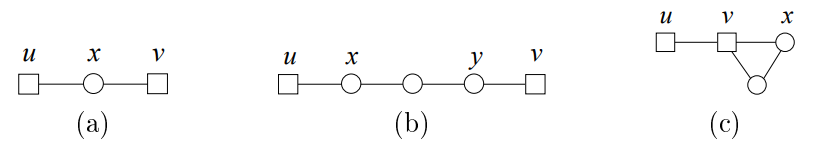
Definition 5.2. For \(v \in V(G)\) and \(r \in \mathbb{N}_0\), let \(T_r(v)\) denote the set of terminal vertices among all trails (i.e., walks which forbid repeated edges) of length \(r\) starting from \(v\).
Observation 5.3. Let \(S\) be a DET:OLD set on cubic graph \(G\). For all vertices \(v \in V(G)-S\), we have \(T_2(v) \cup T_4(v) \subseteq S\).
Proof. Assume to the contrary that there exist \(u,v \in V(G)-S\) such that \(u \in T_2(v) \cup T_4(v)\). We know that \(u \neq v\) because \(G\) is \(C_4\)-free due to the existence of DET:OLD. We consider the three non-isomorphic ways to form a length 2 or 4 trail from \(u\) to \(v\) as illustrated in Figure 9. We see that in Figure 9 (a), \(x\) cannot be 2-dominated, in (b), \(x\) and \(y\) cannot be distinguished, and in (c), \(v\) and \(x\) cannot be distinguished. All three cases contradict the existence of \(S\), completing the proof. ◻
Theorem 5.4. Let \(G\) be a \(C_4\)-free cubic graph, and let \(\overline{S} \subseteq V(G)\) such that for all distinct \(u,v \in \overline{S}\), \(u \notin T_2(v) \cup T_4(v)\). Then \(S = V(G) – \overline{S}\) is a DET:OLD on \(G\).
Proof. Let \(u \in V(G)\). We see that for any distinct \(x,y \in N(u)\), \(x \in T_2(y)\). Thus, by assumption it must be that \(|N(u) \cap \overline{S}| \le 1\), implying that \(dom(u) \ge 2\). We now know that all vertices are at least 2-dominated by \(S\). Next, we consider the following three cases depending on the distance between a pair of vertices and show the pair is \(2^{\#}\)-distinguished.
Case 1. Suppose \(u,v \in V(G)\) with \(d(u,v) = 1\).
Because \(G\) is twin-free (due to being a \(C_4\)-free cubic graph) and regular, it must be that \(\exists x \in N(u) – N[v]\) and \(\exists y \in N(v) – N[u]\). Suppose \(\exists w \in N(u) \cap N(v)\). Then we see that \(\forall p \in N[u] \cup N[v]\), \((N[u] \cup N[v]) – \{p\} \subseteq T_2(p) \cup T_4(p)\), implying that \(|(N[u] \cup N[v]) \cap \overline{S}| \le 1\), from which it can be seen that \(u\) and \(v\) must be distinguished. Otherwise, we can assume that \(N(u) \cap N(v) = \varnothing\). If \(u \in \overline{S}\), then \(N(v) – N[u] \subseteq T_2(u) \subseteq S\), so \(v\) is distinguished from \(u\) and we would be done; otherwise we assume \(u \in S\) and by symmetry \(v \in S\). We see that \(|(N(u) – N[v]) \cap \overline{S}| \le 1\), so \(u\) is distinguished from \(v\).
Case 2. Suppose \(u,v \in V(G)\) with \(d(u,v) = 2\), and let \(N(u) \cap N(v) = \{w\}\), as \(G\) is \(C_4\)-free.
Let \(N(u) – N[v] = \{u',u''\}\) and let \(N(v) – N[u] = \{v', v''\}\). We see that \(\forall p \in \{u',u'',v',v''\}\), \(\{u',u'',v',v''\} – \{p\} \subseteq T_2(p) \cup T_4(p) \subseteq S\), which implies that \(|\{u',u'',v',v''\} \cap \overline{S}| \le 1\). Therefore, \(u\) and \(v\) must be distinguished.
Case 3. Suppose \(u,v \in V(G)\) with \(d(u,v) \ge 3\), and let \(N(u) = \{u',u'',u'''\}\) and \(N(v) = \{v',v'',v'''\}\).
We see that for any \(p \in N(u)\), \(\{u',u'',u'''\} – \{p\} \subseteq T_2(p) \subseteq S\). Thus \(u\) and \(v\) must be distinguished, completing the proof. ◻
From Observations 5.1 and 5.3 and Theorem 5.4, we have the following full characterization of DET:OLD in cubic graphs.
Corollary 5.5. Let \(G\) be a cubic graph and \(S \subseteq V(G)\). Then \(S\) is a DET:OLD if and only if \(G\) is \(C_4\)-free and for all distinct \(u,v \in V(G)-S\), \(u \notin T_2(v) \cup T_4(v)\).
The upper bound on \(\textrm{DET:OLD}(G)\) for cubic graphs is known to be \(\frac{45}{46}n\) [12], and we can improve it using Corollary 5.5.
Theorem 5.6. If \(G\) is a cubic graph that permits DET:OLD, then \(\textrm{DET:OLD%}(G) \le \frac{30}{31}\).
Proof. We will show that we can construct a set \(\overline{S}\) with the property that \(\forall v \in V(G)\), \(\exists u \in \overline{S}\) such that \(v \in T_0(u) \cup T_2(u) \cup T_4(u)\). Because \(|T_0(u)| = 1\), \(|T_2(u)| \le 6\), and \(|T_4(u)| \le 24\), this construction will result in a detector set \(S = V(G) – \overline{S}\) with density at most \(\frac{6 + 24}{1 + 6 + 24} = \frac{30}{31}\). Assume to the contrary that we have a maximal \(\overline{S}\) set, but \(\exists x \in V(G)\) such that \(x \notin T_0(u) \cup T_2(u) \cup T_4(u)\) for any \(u \in \overline{S}\), implying that \(x \notin \overline{S}\). Then by Corollary 5.5, we see that \(\overline{S} \cup \{x\}\) still satisfies the requirements of our \(\overline{S}\) set, contradicting maximality of \(\overline{S}\). Therefore, we have a DET:OLD set \(S\) with density at most \(\frac{30}{31}\), completing the proof. ◻
Corollary 5.7. If \(G\) is a cubic graph that permits DET:OLD, then \(\textrm{DET:OLD}(G) \le n – 1\).
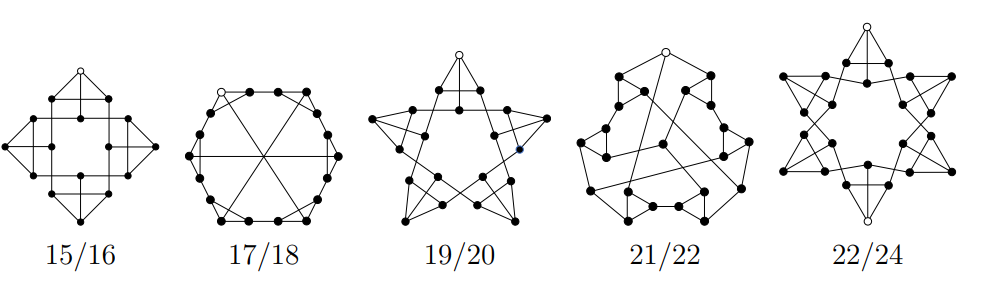
Figure 10 shows extremal cubic graphs with the highest density on \(n\) vertices for \(16 \le n \le 24\). The \(n = 22\) graph shown in Figure 10 has the highest density we have found so far of \(\frac{21}{22}\), and we conjecture the density \(\frac{21}{22}\) is the tight upper bound for all cubic graphs.
In this paper, we have explored various results for minimum-density error-detecting open-locating-dominating (DET:OLD) sets in several classes of graphs. In Theorem 2.3, we discovered that any graph permitting DET:OLD must have \(m \ge \left\lceil \frac{3n – \left\lfloor \frac{n}{2} \right\rfloor}{2} \right\rceil\), and we have constructed an infinite family of graphs on \(n \ge 9\) vertices (shown in Figure 3) which achieves this extremal minimum number of edges. In Theorem 3.4, we found that the decision problem of determining if a general graph permits a DET:OLD of a certain maximum size is NP-complete. Future work could determine if there are any particular classes of graphs for which this problem can be solved in polynomial time. For infinite grids, the minimum density of DET:OLD on HEX, SQR, and TRI is already known; in this paper, we have improved the bounds for KNG to \(\frac{3}{8} \le \textrm{DET:OLD%}(\textrm{KNG}) \le \frac{13}{30}\). Future research may further reduce this gap or determine the exact value of \(\textrm{DET:OLD%}(\textrm{KNG})\).
For cubic graphs, Observation 5.1 revealed that DET:OLD exists if and only if \(G\) is \(C_4\)-free. In Theorem 5.6, we demonstrated that any cubic graph permitting DET:OLD must have \(\textrm{DET:OLD%}(G) \le \frac{30}{31}\). In Figure 10, we have provided a collection of cubic graphs on \(16 \le n \le 24\) vertices with the highest minimum density of DET:OLD. Future work could extend this to an infinite family and discover whether the \(\frac{30}{31}\) upper bound is tight. However, from computer-assisted exploration, we believe this \(\frac{30}{31}\) bound is not tight and instead propose the following conjecture:
Conjecture 6.1. If \(G\) is a cubic graph permitting DET:OLD, then \(\textrm{DET:OLD%}(G) \le \frac{20}{21}\).