
Graph decompositions have been extensively studied for decades and became one of the classical themes in graph theory. Decomposition of complete graphs into mutually isomorphic subgraphs is probably the most popular topic within this area. We say that a graph \(G\) decomposes \(K_n\) if there exist subgraphs \(G_1,G_2,\dots, G_s\) of \(K_n\), all isomorphic to \(G\), such that every edge of \(K_n\) appears in exactly one copy \(G_i\) of \(G\). One selects a class of graphs \(\mathcal{G}\), finite or infinite, and finds complete graphs that admit a decomposition into all graphs in \(\mathcal{G}\). Such a collection of complete graphs is then called the spectrum of \(\mathcal{G}\).
In this paper we continue the effort to find the spectrum for all graphs with a given (small) number of edges by determining which complete graphs they decompose. Almost all graphs with up to six edges have been fully classified, as well as almost all graphs with eight edges. For a detailed overview, we refer the reader to Adams, Bryant, and Buchanan [1]. For graphs with seven edges, much less is known. An overview of known results is presented in Section 2.
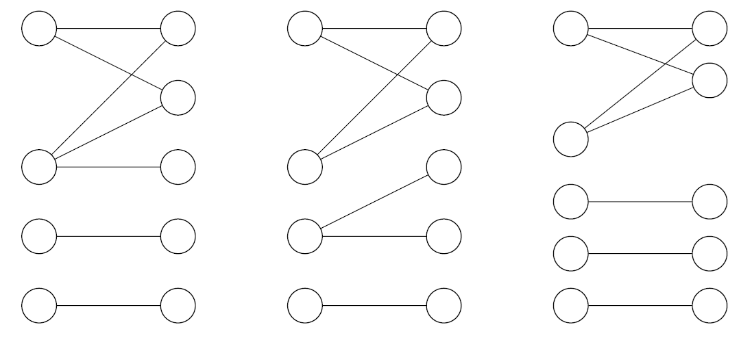
We continue in this direction by determining the spectrum for all disconnected unicyclic bipartite graphs with seven edges and nine or ten vertices decomposing complete graphs. A unicyclic graph is a simple finite graph without loops containing exactly one cycle. There are three such graphs, either with three or four components. We call them \(G_1, G_2, G_3\) and denote \(\mathcal{G}=\{G_i\mid i=1,2,3\}\). They are presented in Figure 1.
The obvious necessary condition for \(K_n\) to be decomposable into a graph with seven edges is \(n\equiv0,1\pmod7\).
For \(n\equiv0,1\pmod{14}\) the decompositions are based on Rosa-type labelings, introduced by Rosa in 1967 [13]. This is done in Section 4. In Section 5 for \(n\equiv7\pmod{14}\) we decompose \(K_n\) first into graphs \(K_{7,7}\) and \(K_{14}-K_7\) and then each of them into the desired graph \(G_i\) using again mostly labeling techniques. Finally, in Section 6 for \(n\equiv8\pmod{14}\), we use labeling techniques with two different starters.
Disclaimer. Since this paper is a direct continuation of paper [10] by the third author and Kubesa, some parts of Sections 1, 2, and 3 are similar or identical to those in [10].
For an excellent survey on \(G\)-designs, we refer the reader to [1]. There is a thorough section on graphs with at most six vertices, which covers a good number of graphs with seven edges.
For graphs with at most six edges and those with eight edges the spectrum is almost completely known except for a small number of cases; the class of graphs with seven edges is still wide open.
Graphs with seven edges and five vertices are always connected and the spectrum was determined by Bermond, Huang, Rosa, and Sotteau [4] with 11 possible exceptions. Five of them for \(K_5 – K_{1,3}\) were constructed by Chang [7]. For \(K_5 – (P_3\cup P_2)\), five were constructed by Li and Chang [12] and the remaining one by Adams, Bryant, and Buchanan [1].
Theorem 2.1 (Bermond et al. [4], Chang [7], Li and Chang [12], Adams, Bryant, and Buchanan [1]). There exists a \(G\)-decomposition of \(K_{n}\) for a graph \(G\) on seven edges and five vertices if and only if
1. \(G=K_5-K_{1,3}, n\equiv0,1\pmod7, n\geq 14\), or
2. \(G=K_5-K_{3}, n\equiv1,7\pmod{14},\) or
3. \(G=K_5-(P_{3}\cup P_2), n\equiv0,1\pmod7, n\neq8,14\), or
4. \(G=K_5-(P_{4}), n\equiv0,1\pmod7, n\neq8\).
Blinco [5] and Tian, Du, and Kang [14] studied connected graphs with seven edges and six vertices. The only disconnected graph with seven edges and six vertices is \(K_4\cup K_2\) and the spectrum for this graph was also found in [14].
Theorem 2.2(Blinco [5], Tian et al. [14]).There exists a \(G\)-decomposition of \(K_{n}\) for a graph \(G\) on seven edges and six vertices if and only if \(n\equiv0,1\pmod7\) except for eight exceptions when \(n=7\) or \(n=8\).
All graphs with seven edges and seven vertices are either connected and unicyclic or disconnected. A complete solution for connected bipartite (and necessarily unicyclic) graphs was obtained by Froncek and Kubesa in [9].
Theorem 2.3(Froncek, Kubesa [9]).There exists a \(G\)-decomposition of \(K_{n}\) for a connected bipartite unicyclic graph \(G\) on seven edges and seven vertices if and only if \(n\equiv0,1\pmod7\) except for three exceptions when \(n=7\) and two exceptions when \(n=8\).
The only remaining connected class for seven edges and seven vertices is then unicyclic tripartite graphs. To our knowledge, this class has not received any attention yet.
Since the solution is not covering the whole spectrum, we pose our first open problem.
Problem 2.4. Complete the \(G\)-decomposition spectrum for connected tripartite graphs on seven edges and seven vertices (which are necessarily unicyclic).
We do not know any result on the spectrum of disconnected graphs with seven edges and seven vertices. Our second open problem is then the following.
Problem 2.5. Determine the \(G\)-decomposition spectrum for disconnected graphs on seven edges and seven vertices.
Connected graphs with seven edges and eight vertices are trees, which were investigated by Huang and Rosa [11].
Theorem 2.6(Huang, Rosa [11]). There exists a \(G\)-decomposition of \(K_{n}\) for a connected graph \(G\) on seven edges and eight vertices (that is, a tree) if and only if \(n\equiv0,1\pmod7, n\geq 8\) except for nine exceptions when \(n=8\).
For disconnected bipartite graphs with seven edges and eight vertices, a complete solution was obtained by Froncek and Kubesa in [10].
Theorem 2.7 (Froncek, Kubesa [10]). There exists a \(G\)-decomposition of \(K_{n}\) for a disconnected bipartite unicyclic graph \(G\) on seven edges and eight vertices if and only if \(n\equiv0,1\pmod7, n\geq 8\) with three exceptions when \(n=8\).
In this paper we completely determine the spectrum for disconnected unicyclic bipartite graphs on seven edges by solving the cases with nine or ten vertices.
The remaining graphs with seven edges and more than seven vertices are necessarily disconnected. The spectrum for forests was completely determined by Banegas and Freyberg [3].
Theorem 2.8(Banegas, Freyberg [3]). There exists a \(G\)-decomposition of \(K_{n}\) for a forest \(G\) on seven edges if and only if \(n\equiv0,1\pmod7, n\geq14\).
A partial result for unicyclic ones was obtained recently by Banegas et al. [2].
Theorem 2.9(Benagas et al. [2]). There exists a \(G\)-decomposition of \(K_{n}\) for a disconnected tripartite unicyclic graph \(G\) on seven edges whenever \(n\equiv0,1\pmod{14}, n\geq 14\).
This leaves us with the third open problem.
Problem 2.10. Complete the \(G\)-decomposition spectrum for disconnected graphs on seven edges and more than seven vertices.
The following definition has been used in different variations for years, and we present it just for the sake of completeness.
Definition 3.1. Let \(H\) be a graph. A decomposition of the graph \(H\) is a collection of pairwise edge-disjoint subgraphs \(\mathcal{D}=\{G_1,G_2,\dots,G_s\}\) such that every edge of \(H\) appears in exactly one subgraph \(G_i\in\mathcal{D}\).
We say that the collection forms a \(G\)-decomposition of \(H\) (also known as an \((H,G)\)-design) if each subgraph \(G_i\) is isomorphic to a given graph \(G\). If \(H\) is the complete graph \(K_n\), then we can use just the term \(G\)-design.
Because we focus solely on decompositions of complete graphs, we only use the term \(G\)-decomposition or \(G\)-design. The following definition was used by Rosa [13] already in 1967. We are unsure whether this was the first appearance of that definition though.
Definition 3.2. A \(G\)–decomposition of the complete graph \(K_n\) is cyclic if there exists an ordering \((x_0,x_1,\dots, x_{n-1})\) of the vertices of \(K_n\) and a permutation \(\varphi\) of the vertices of \(K_n\) defined by \(\varphi(x_j)=x_{j+1}\) for \(j=0,1,\dots,n-1\) inducing an automorphism on \(\mathcal{D}\), where the addition is performed modulo \(n\).
As above, we are not sure when the following definition was stated first time using the exact terminology. A construction using this type of decomposition was used already by Huang and Rosa [11] in 1978.
Definition 3.3. A \(G\)–decomposition of the complete graph \(K_n\) is \(1\)-rotational if there exists an ordering \((x_0,x_1,\dots, x_{n-1})\) of the vertices of \(K_n\) and a permutation \(\varphi\) of the vertices of \(K_n\) defined by \(\varphi(x_j)=x_{j+1}\) for \(j=0,1,\dots,n-2\) and \(\varphi(x_{n-1})=x_{n-1}\) inducing an automorphism on \(\mathcal{D}\), where the addition is performed modulo \(n-1\).
We will use the interval notation \([k,n]\) for the set of consecutive integers \(\{k,k+1,k+2,\dots,n\}\). When \(k=1\), the interval is denoted simply by \([n]\).
One of the basic and most useful tools for finding \(G\)-designs is the following labeling.
Definition 3.4(Rosa [13]).Let \(G\) be a graph with \(n\) edges. A \(\rho\)-labeling (sometimes also called rosy labeling) of \(G\) is an injective function \(f\colon V(G)\rightarrow[0,2n]\) that induces the length function \(\ell\colon E(G)\rightarrow[n]\) defined as \[\ell(uv)=\min\{|f(u)-f(v)|,2n+1-|f(u)-f(v)|\},\] with the property that \[\{\ell(uv):uv\in E(G)\}=[n].\]
A graph \(G\) possessing a \(\rho\)-labeling decomposes the complete graph, as proved by Rosa in 1967.
Theorem 3.5(Rosa [13]). Let \(G\) be a graph with \(n\) edges. A cyclic \(G\)-decomposition of the complete graph \(K_{2n+1}\) exists if and only if \(G\) admits a \(\rho\)-labeling.
When a graph \(G\) with \(n\) edges has a vertex \(w\) of degree one and \(G-w\) admits a \(\rho\)-labeling, a modification of \(\rho\)-labeling can be used to find a \(G\)-decomposition of \(K_{2n}\). Such labeling is known as \(1\)-rotational \(\rho\)-labeling and was first used by Huang and Rosa in [11], although a formal definition was not stated there.
Definition 3.6(Huang, Rosa [11]). Let \(G\) be a graph with \(n\) edges and edge \(ww'\) where \(\deg(w)=1\). A \(1\)-rotational \(\rho\)-labeling of \(G\) consists of an injective function \(f\colon V(G)\rightarrow[0,2n-2]\cup\{\infty\}\) with \(f(w)=\infty\) that induces a length function \(\ell\colon E(G)\rightarrow[n-1]\cup \{\infty\}\) which is defined as \[\ell(uv)=\min\{|f(u)-f(v)|,2n-1-|f(u)-f(v)|\},\] for \(u,v\neq w\) and \[\ell(ww')=\infty\] with the property that \[\{\ell(uv):uv\in E(G)\}=[n-1]\cup\{\infty\}.\]
This technique was used in [11] and proved only for particular graphs studied in that paper. The following theorem is considered folklore.
Theorem 3.7. Let \(G\) be a graph with \(n\) edges. If \(G\) admits a \(1\)-rotational \(\rho\)-labeling, then there exists a \(1\)-rotational \(G\)-decomposition of the complete graph \(K_{2n}\).
As we observed before, a necessary condition for \(K_{n}\) to admit a \(G\)-design for a graph \(G\) with 7 edges is that the number of edges in \(K_{n}\) must be divisible by 7, implying \(n\equiv0,1\pmod{7}\). For the graphs we are interested in, the above theorems only allow decompositions of \(K_{14}\) and \(K_{15}\). Therefore, we will need additional tools, which are some more restrictive modifications of \(\rho\)-labeling yet also produce \(G\)-decompositions of larger complete graphs; that is, \(K_{2nk+1}\) for any \(k\geq1\) when \(G\) has \(n\) edges.
Definition 3.8(El-Zanati, Vanden Eynden, Punnim [16]).Let \(G\) be a bipartite graph with \(n\) edges and a vertex bipartition \(U\cup V\). A \(\rho^+\)-labeling of \(G\) is a \(\rho\)-labeling \(f\) with the additional property that for every \(u\in U\) and \(v\in V\) if \(uv\in E(G)\), then \(f(u)<f(v)\). A \(\sigma^+\)-labeling is a \(\rho^+\)-labeling without wrap-around edges, that is, the length function is defined as \[\ell(uv)=f(v)-f(u).\]
These conditions guarantee decompositions of \(K_{2nk+1}\), as proved by El-Zanati, Vanden Eynden and Punnim [16].
Theorem 3.9(El-Zanati, Vanden Eynden, Punnim [16]). Let \(G\) be a bipartite graph with \(n\) edges. If \(G\) admits a \(\rho^+\)-labeling or a \(\sigma^+\)-labeling, then there exists a cyclic \(G\)-decomposition of the complete graph \(K_{2nk+1}\) for every \(k\geq1\).
Notice that mentioning the \(\sigma^+\)-labeling in Theorem 3.9 is in fact redundant, because every \(\sigma^+\)-labeling is a \(\rho^+\)-labeling. We mention it there explicitly for clarity because in what follows we will be only using \(\sigma^+\)-labeling in our constructions.
To decompose complete graphs with \(2nk\) vertices into graphs with \(n\) edges, we will use the \(1\)-rotational \(\sigma^+\)-labeling.
Definition 3.10. Let \(G\) be a bipartite graph with \(n\) edges, vertex \(w\) of degree one and an edge \(ww'\). A \(1\)-rotational \(\sigma^+\)-labeling of \(G\) is a \(1\)-rotational \(\rho\)-labeling with the additional property that for every \(u\in U\) and \(v\in V\) if \(u,v\neq w\) and \(uv\in E(G)\), then \(f(u)<f(v)\) and the length function is defined as \[\ell(uv)=f(v)-f(u),\] for \(u,v\neq w\), \[f(w)=\infty, \ \text{and} \ \ \ell(ww')=\infty.\]
The following analogues of the above theorems were proved recently. Bunge [6] proved the following.
Theorem 3.11(Bunge [6]).Let \(G\) be a bipartite graph with \(n\) edges and with \(w\in V(G)\) such that \(\deg(w)=1\). If \(G- w\) admits a \(\rho^{+}\)-labeling, then there exists a \(1\)-rotational \(G\) decomposition of \(K_{2nk}\) for any positive integer \(k\).
It is easy to see that when we have a \(\sigma^+\)-labeling where the longest edge is \(ww'\), vertex \(w\) is of degree one and all other vertices have labels at most \(2n-2\), the labeling can be transformed to a \(1\)-rotational \(\sigma^+\)-labeling.
The following theorem is more restrictive in the labeling properties but allows us to use the same labeling for \(G\)-decompositions of both \(K_{2nk+1}\) and \(K_{2nk}\).
Theorem 3.12(Fahnenstiel, Froncek [8]).Let \(G\) be a bipartite graph with \(n\) edges and a vertex of degree one. If \(G\) admits a \(\sigma^+\)-labeling with the additional property that the edge of length \(n\) is pendant and no vertex label is greater than \(2n-2\), then there exists a cyclic \(G\)-decomposition of the complete graph \(K_{2nk+1}\) and a \(1\)-rotational \(G\)-decomposition of the complete graph \(K_{2nk}\) for every \(k\geq1\).
In our constructions, we will also need to decompose complete bipartite graphs. The tools are similar, based on labelings as well. An equivalent of \(\rho\)-labeling for bipartite graphs is called bilabeling and has been used for years by numerous authors. The following definition is adapted from [15].
Definition 3.13. Let \(G\) be a bipartite graph with \(n\) edges and a vertex bipartition \(U\cup V\). A
\(\rho\)-bilabeling of \(G\) is a function \(f:V(G)\to[0,n-1]\) that is injective when restricted to sets \(U\) and \(V\) and the induced length function defined as \[\ell(uv)=(f(v)-f(u))\hspace{-10pt}\pmod{n},\] has the property that \[\{\ell(uv):uv\in E(G)\}=[0,n-1].\]
The following theorem was proved in a simpler form independently by many authors; e.g., in [15].
Theorem 3.14. Let \(G\) be a bipartite graph with \(n\) edges. If \(G\) admits a \(\rho\)-bilabeling, then there exists a \(G\)-decomposition of the complete bipartite graph \(K_{nk,nm}\) for every \(k,m\geq1\).
Our decompositions of \(K_n\) for \(n\equiv1\pmod{14}\) are based on \(\sigma^+\)-labelings of the respective graphs.
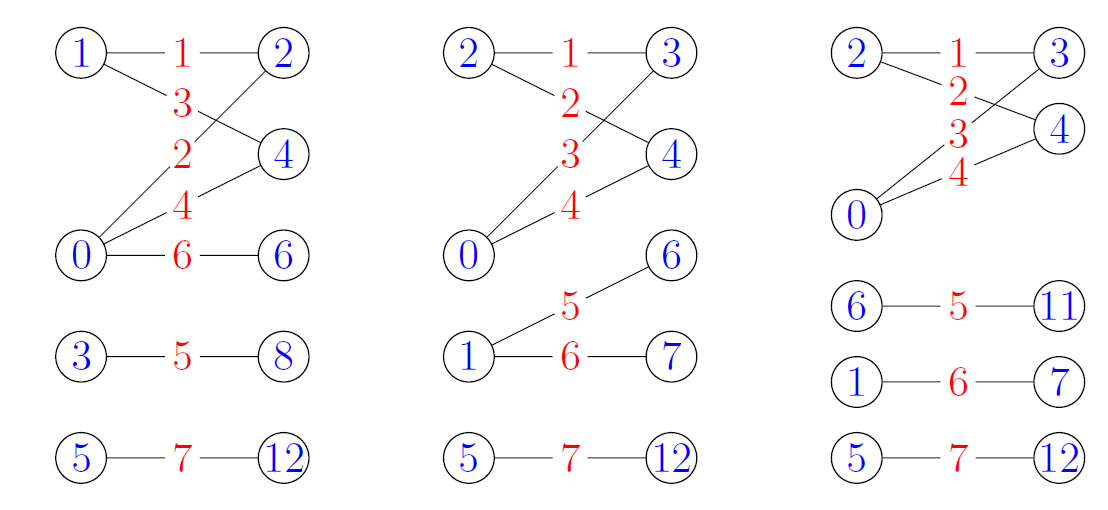
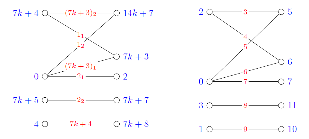
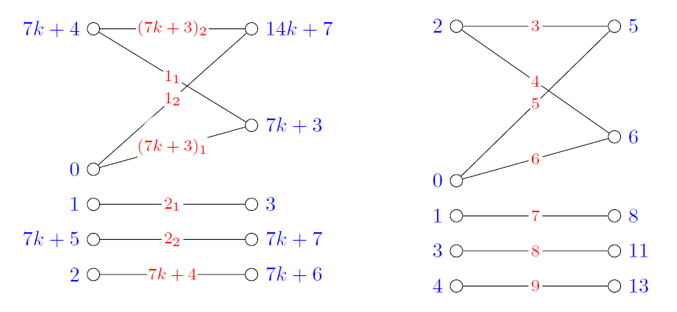
Theorem 4.1. There exists a \(G_i\)-decomposition of the complete graph \(K_{14k}\) and \(K_{14k+1}\) into each graph \(G_i\in\mathcal{G}\) for every \(k\geq1\).
Proof. Each graph \(G_i\in\mathcal{G}\) has a \(\sigma^+\) labeling shown in Figure 2, with no vertex label bigger than \(2n-2=12\). The longest edge of length 7 is pendant with one endvertex labeled \(12\). Therefore, a decomposition exists by Theorem 3.12. ◻
In this case, we let \(n=14k+7\) and first decompose \(K_{14k+7}\) into \(2k+1\) graphs \(K_{14}-K_7\) and \((k-1)(2k+1)\) copies of \(K_{7,7}\). Then we use it to find a \(G\)-decomposition of \(K_{14k+7}\).
We first partition the vertex set of \(K_{14k+7}\) into \(2k+1\) sets \(X_i, i=1,2,\dots,2k+1\), where \(X_i=\{x_{i,0},x_{i,1},\dots,x_{i,6}\}\). Then we take the complete bipartite graph \(K_{7,7}\) with partite sets \(X_i\) and \(X_{i+1}\) (and with \(X_{2k+1}\) and \(X_1\) when \(i=2k+1\)) and add the edges of the complete graph \(K_7\) induced on \(X_i\) to obtain our graphs \(K_{14}-K_7\). We denote these graphs \(H_i\) where the index \(i\) corresponds the index of \(X_i\) which is filled by \(K_7\). For the remaining pairs of sets \(X_i,X_j, \ i,j\in \{1,2,\dots,2k+1\}, j\neq i, j\neq i\pm1\), again computed modulo \(2k+1\), we obtain the graphs \(K_{7,7}\) with bipartition \(X_i,X_j\).
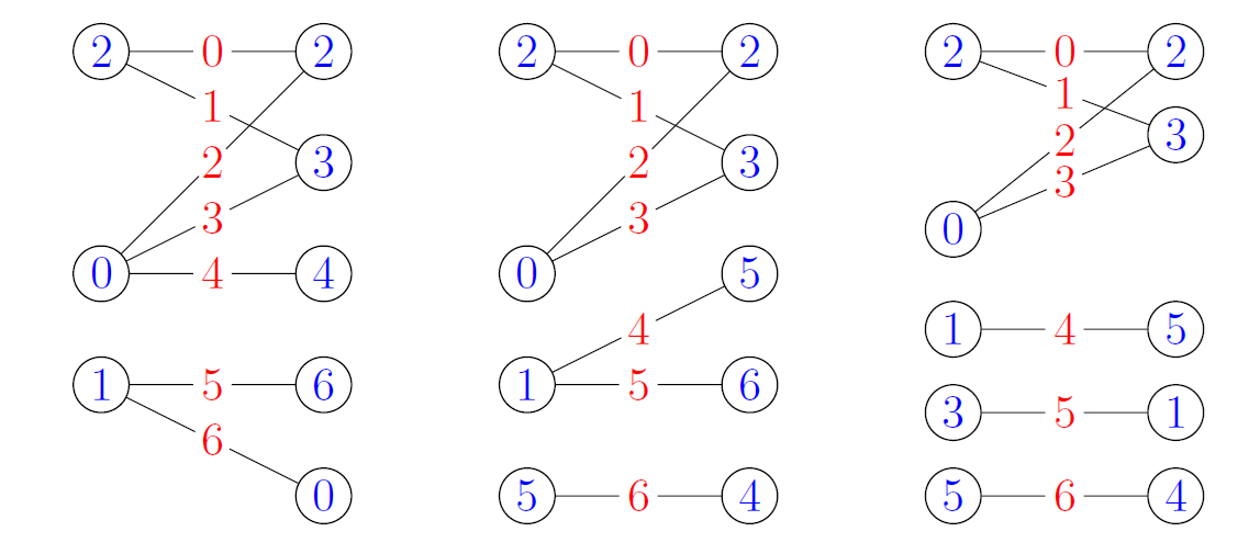
To show that \(K_{7,7}\) is \(G\)-decomposable, it is enough to find a \(\rho\)-bilabeling of \(G\). They are shown in Figure 3.
A lemma follows immediately.
Lemma 5.1. The complete bipartite graph \(K_{7,7}\) is \(G\)-decomposable for every \(G\in\mathcal{G}\).
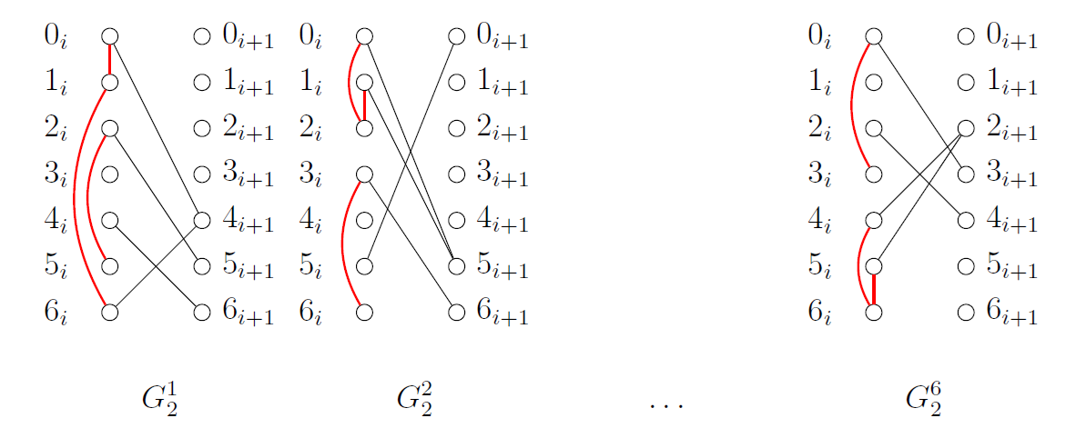
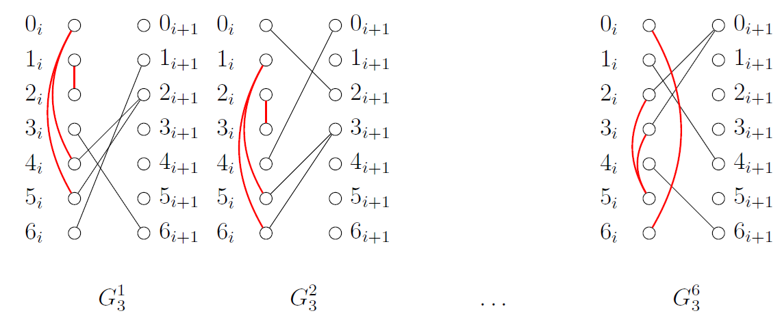
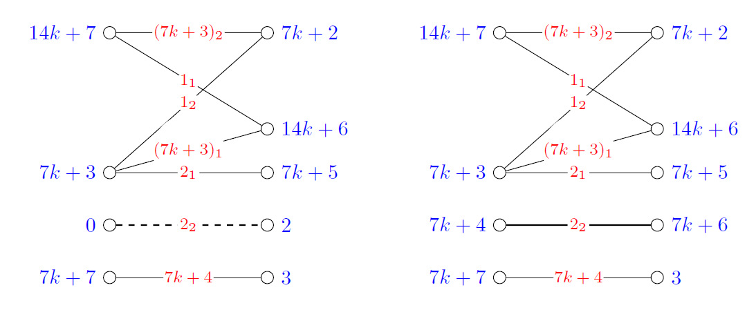
Construction 5.2. In Figure 4 we show a \(G_1\)-decomposition of the graph \(H_i\cong K_{14}-K_7\). A vertex \(x_{i,j}\) is depicted as \(j_i\), where \(j\) is also the label.
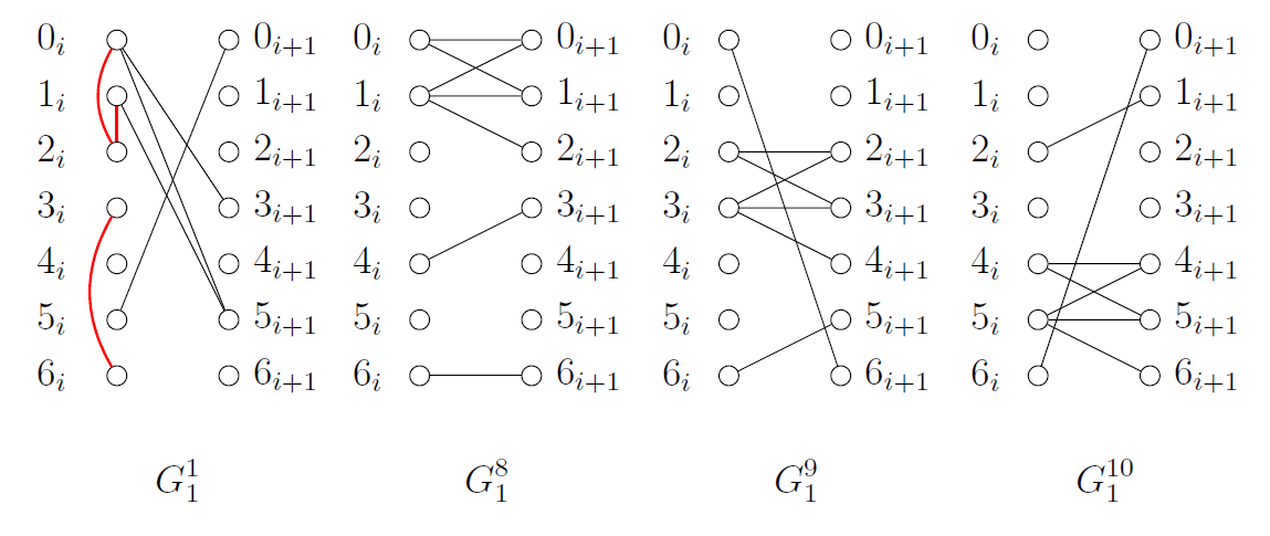
The edge lengths are calculated in two different ways depending on whether the edge belongs to \(K_7\) or \(K_{7,7}\). The edges in \(K_7\) are red and the length is calculated as in \(\rho\)-labeling, that is \[\ell(x_{i,a}x_{i,b}) = \ell(a_i b_i) = \min\{|a-b|, 7-|a-b|\}.\] One can observe that the lengths in \(G_1^1\) with respect of the complete graph \(K_7\) induced on \(X_i\) are in \([3]\) and thus satisfy the conditions on \(\rho\)-labeling of a graph with three edges.
In \(K_{7,7}\) the edges are black and we use a \(\rho\)-bilabeling with edge lengths \[\ell(x_{i,a}x_{i+1,b}) = \ell(a_i b_{i+1}) = (b-a)\!\!\!\mod7.\]
Again in \(G_1^1\) the bilabeling lengths are \([2,5]\). Rotating the graphs \(G_1^1\) with step one seven times, we use all edges of these lengths. Here by a rotation with step \(t\) we mean a permutation \(\varphi(x_{i,j}) = x_{i,j+t}\) where the addition in the second subscript is performed modulo 7. The other 21 edges with bilabeling lengths 0, 1, and 6, are used for the remaining copies \(G_1^8,G_1^9,G_1^{10}\).
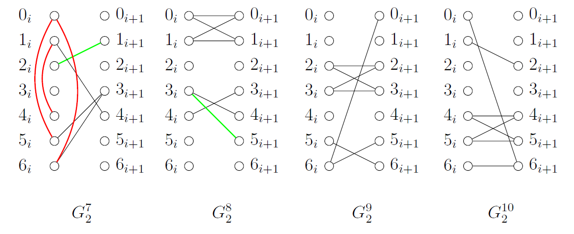
Construction 5.3. For a \(G_2\)-decomposition of \(H_i\cong K_{14}-K_7\), we rotate the graph \(G_2^1\) shown in Figure 5 only six times. This is so because we need to “borrow” one edge from the seventh rotation and place it to what will be the graph \(G_2^8\). Namely, the edge \(3_i5_{i+1}\) will be placed in \(G_2^8\) and replaced by \(2_i1_{i+1}\). The edges are colored green in Figure 6. We need this adjustment because it is impossible to find three copies of \(G_2\) made up form edges of lengths \(0, 1\) and \(6\) between the two partite sets of the partition.
Construction 5.4. Similarly as in Construction 5.3, we rotate the graph \(G_2^1\) shown in Figure 5 only six times. This time we “borrow” the edge \(0_i1_i\) from the seventh rotation and place it to what will be the graph \(G_2^9\). Then the edge \(0_i6_{i+1}\) will be placed in \(G_2^7\) for the same reasons as in the previous construction. It is in Figure 8 colored green again.
The construction immediately yield our next lemma.
Lemma 5.5. The graph \(K_{14}-K_7\) is \(G\)-decomposable for every \(G\in\mathcal{G}\).
Proof. The decompositions are shown in Figures 4–8 and explained in Constructions 5.2–5.4. ◻
Theorem 5.6. The complete graph \(K_{14k+7}\) is \(G\)-decomposable for every graph \(G\in\mathcal{G}\) if and only if \(k\geq1\).
Proof. First we recall that \(K_{14k+7}\) is decomposable into \(2k+1\) copies of \(K_{14}-K_{7}\) and \((k-1)(2k+1)\) copies of \(K_{7,7}\).
Each \(K_{7,7}\) is \(G\)-decomposable by Lemma 5.1 while \(K_{14}-K_{7}\) is \(G\)-decomposable by Lemma 5.5. The condition \(k\geq1\) is obvious. ◻
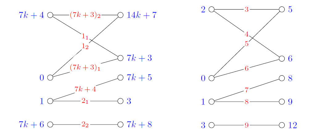
In this case, we will use another method based on \(\sigma^+\)-type labeling. Because the number of different edge lengths in \(K_{14k+8}\) is not a multiple of seven, we will need two different starters. One will use edge lengths 1, 2, and \(7k+3\), each of them twice, and length \(7k+4\) once. This is so because there are \(7k+8\) edges of each length \(1,2,\dots,14k+3\) but only \(7k+4\) edges of length \(7k+4\). We call this starter \(G^1_i\); the other starter consists of graphs \(G_i^2,G_i^3,\dots,G_i^{k+1}\). Labelings of \(G_i^1\) and \(G_i^2\) are shown in Figures 9–13.
By rotation with step \(t\) we mean the mapping \(i\mapsto i+t\) for every \(i\in[0,14k+7]\) computed modulo \(14k+8\).
The starter \(G_1^1\) will be rotated with step one \(7k+4\) times, covering all \((7k+4)(3\cdot2 + 1) = 49k + 28\) edges of lengths \(1, 2, 7k+3\) and \(7k+4\). Then \(k\) starters \(G_1^2,G_1^3,\dots,G_1^{k+1}\) contain edges of seven different lengths each and will be rotated with step one \(14k+8\) times, covering \(7k(14k+8) = 98k^2 + 56k\) edges of lengths \(3,4,\dots,14k+3\). Therefore, we cover \[\begin{aligned} (49k + 28)+(98k^2 + 56k) &= (49k + 28)(2k+1) \\ &= 7(7k+4)(2k+1)\\ &= (7k+4)(14k+7)\\ &= (14k+8)(14k+7)/2, \end{aligned}\] edges, which is exactly the number of edges in \(K_{14k+8}\).
Construction 6.1. In the graph \(G_1^1\), let \(uv\) be an edge of length \(a\) and \(f(v) = f(u)+a\) where the addition is performed modulo \(14k+8\). Then we call the vertex \(u\) the leading vertex. For edges with the same length, the one with the smaller leading vertex label has the subscript 1 and the other one subscript 2. The subscript will not change even when in some of the following copies the labels will be ordered conversely.
We label \(G_1^1\) as in Figure 9 and rotate it with step one, obtaining \(7k+4\) copies. The edges of length 1 have the leading vertices \(7k+3\) and \(14k+7\), therefore are exactly \(7k+4\) rotations with step one apart. Hence, after \(7k+4\) rotations with step one, the \(7k+4\) copies of \(G_1^1\) do not repeat an edge of length 1. Similarly, the edges of length \(7k+3\) have leading vertices 0 and \(7k+4\) and the same argument applies.
However, the leading vertices of edges of length 2 are 0 and \(7k+5\) and therefore differ by \(7k+3\) rotations with step one only. This means that without an adjustment, the edge \((0,2)\) has images \((0,2),(1,3),\dots,(7k+3,7k+5)\) while \((7k+5,7k+7)\) has images \((7k+5,7k+7),(7k+6,7k+8),\dots,(0,2)\). In particular, the edge \((0,2)\) is used twice while \((7k+4,7k+6)\) not at all. Hence, in the \((7k+4)\)-th copy of \(G_1^1\) we use the edge \((7k+4,7k+6)\) instead of \((0,2)\), as shown in Figure 10.
Finally, the only edge of length \(7k+4\) is \((4,7k+8)\) and we have used every edge of length \(1, 2, 7k+3\) and \(7k+4\) exactly once.
For the other starter, a labeling of \(G_1^2\) is shown in Figure 9. For the remaining graphs \(G_1^j, j=2,\dots,k+1\) we define the labeling recursively. Let the vertices in the partite set \(X\) (with the smaller labels) be \(x_s\) and in the partite set \(Y\) (with the higher labels) be \(y_t\). Denote the labeling function \(f\) piecewise, where \(f_j\) is the labeling for the graph \(G_1^j\). Function \(f_2\) is shown in Figure 9. For \(j=3,4,\dots,k+1\) we define \[f_j(x_s) = f_{j-1}(x_s),\] and \[f_j(y_t) = f_{j-1}(y_t)+7.\]
This way every graph \(G_1^j\) in the starter contains seven consecutive lengths, \(7(j-2)+3,7(j-2)+4,\dots,7(j-2)+9\).
Each \(G_1^j\) will now be rotated with step one \(14k+8\) times. Hence, every edge of \(K_{14k+8}\) appears in exactly one rotated copy of some \(G_1^j\) and thus we have a valid \(G_1\)-decomposition.
Construction 6.2. The construction of \(G_2^1\) is essentially the same as in Construction 6.1.
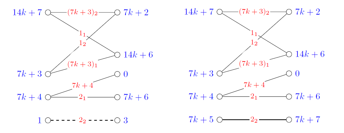
We label \(G_2^1\) as in Figure 11 and rotate it again with step one. The edges of length 1 and \(7k+3\) behave exactly the same as in Construction 6.1.
The leading vertices of edges of length 2, namely 1 and \(7k+6\), differ again by \(7k+3\) rotations with step one only. The edge \((1,3)\) has images \((1,3),(2,4),\dots,(7k+2,7k+4)\) while \((7k+6,7k+8)\) has images \((7k+6,7k+8),(7k+7,7k+9),\dots,(1,3)\). The edge \((1,3)\) is used twice while \((7k+5,7k+7)\) not at all. Hence, in the \((7k+4)\)-th copy of \(G_2^1\) we use the edge \((7k+5,7k+7)\) instead of \((1,3)\).
Finally, the only edge of length \(7k+4\) is \((1,7k+5)\) and we have used every edge of the four used lengths exactly once.
The rest of the construction is identical to Construction 6.1.
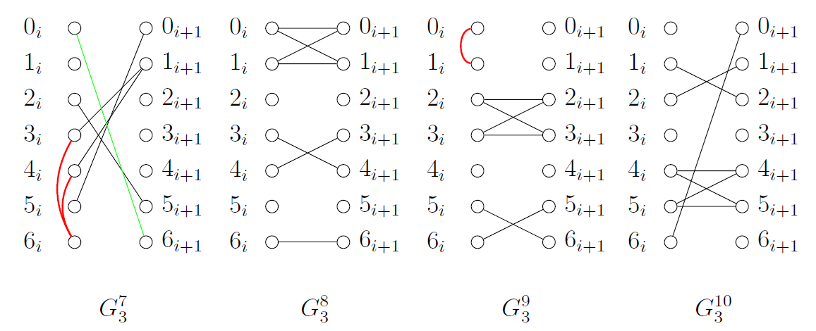
Construction 6.3. The construction of \(G_3^1\) is even simpler than the previous two. It is so because for all three pairs of edges of the same length, \(1, 2\), and \(7k+3\) we are able to place the same-length edges at distance \(7k+4\) apart and no edge of the complete graph is used twice (or not at all). A labeling is shown in Figure 13. The rest of the construction is identical to the previous two.
We now again have all ingredients needed for the complete result on this subclass for \(n\equiv8\pmod{14}\).
Theorem 6.4. The complete graph \(K_{14k+8}\) is \(G\)-decomposable for every graph \(G\in\mathcal{G}\) if and only if \(k\geq1\).
Proof. Follows directly from Constructions 6.1–6.3 and the fact that the graphs have more than eight vertices. ◻
Our main result now follows.
Theorem 7.1. The complete graph \(K_n\) has a \(G\)-decomposition for any \(G\in\mathcal{G}\) if and only if \(n\equiv0,1\pmod7, n>8\).
Proof. The case of \(n\equiv0,1\pmod{14}\) is covered by Theorem 4.1. The case of \(n\equiv7\pmod{14}\) is proved in Theorem 5.6 and for \(n\equiv8\pmod{14}\) in Theorem 6.4. ◻
We now combine our result with previous results by Froncek and Kubesa stated in Theorems 2.3 and 2.7 to obtain the complete spectrum for bipartite unicyclic graphs on seven edges.
Theorem 7.2. The complete graph \(K_n\) has a \(G\)-decomposition for any bipartite unicyclic graph on 7 edges if and only if \(n\equiv0,1\pmod7\) and \(n\geq|V(G)|\) except for three exceptions when \(n=7\) and five exceptions when \(n=8\) (two connected and three disconnected).
The authors would like to thank the anonymous referees for their detailed comments and suggestions that helped to significantly improve the paper.