
Graph labelling and graph colouring are closely related themes in structural graph theory. In a proper vertex colouring, adjacent vertices receive distinct colours, whereas a graph labelling assigns numerical labels to vertices or edges subject to prescribed conditions. In many labelling problems the labels induce a colouring through a local rule, and the principal question is to determine the smallest label set that makes the induced colouring proper.
The vertex version of gap labelling was introduced by Dehghan, Sadeghi and Ahadi in their study of the algorithmic complexity of proper labelling problems [5]. In a gap-\([q]\)-vertex labelling, the colour of a vertex of degree at least two is the difference between the largest and smallest labels appearing in its neighbourhood. The associated decision problems are computationally difficult in general. In particular, deciding whether a graph admits a gap-\([q]\)-vertex labelling is NP-complete for fixed \(q\geq3\), and restrictive variants remain NP-complete for \(q=2\) [5, 4]. Structural results are nevertheless available for several classical graph families. Weffort-Santos, Campos and Schouery studied cycles, crowns, wheels, unicyclic graphs and several related families, and developed further structural and algorithmic results for proper gap labellings [7].
The Petersen graph is one of the most prominent cubic graphs and appears throughout graph theory as a canonical example and counterexample [3]. Its generalization, the family of generalized Petersen graphs, was named and systematically studied by Watkins [6]. These graphs have subsequently been investigated from many viewpoints, including Hamiltonicity and extremal structure [1, 2]. Their uniform cubic structure and explicit cyclic description make them a natural setting in which to study neighbourhood-based labellings.
The purpose of this paper is to determine the vertex-gap number for several broad classes of generalized Petersen graphs. Our first result completely settles the gap-\([2]\) case: a generalized Petersen graph admits a gap-\([2]\)-vertex labelling exactly when it is bipartite. We then give explicit gap-\([3]\)-vertex labellings for six non-bipartite parameter families. The constructions are expressed in modular or block form, and in each proof we verify the induced colours on the outer edges, the spokes and the inner edges. The paper concludes with a conjectural classification of the remaining cases.
Throughout the paper, all graphs are finite, simple and undirected. For a graph \(G\), the vertex and edge sets are denoted by \(V(G)\) and \(E(G)\), respectively. The neighbourhood and degree of a vertex \(v\) are denoted by \(N(v)\) and \(d(v)\).
To avoid a conflict with the parameter \(k\) in the generalized Petersen graph \(P(n,k)\), we use \(q\) for the number of available labels.
Definition 2.1. Let \(q\) be a positive integer. A gap-\([q]\)-vertex labelling of a graph \(G\) is a pair \((f,C_f)\), where \[f:V(G)\longrightarrow\{1,2,\ldots,q\},\] and \(C_f\) is the induced vertex colouring defined by \[C_f(v)= \begin{cases} 1, & d(v)=0,\\ f(u), & N(v)=\{u\},\\ \displaystyle \max_{u\in N(v)}f(u)-\min_{u\in N(v)}f(u), & d(v)\geq2, \end{cases}\] such that \(C_f\) is a proper vertex colouring of \(G\). The minimum \(q\) for which \(G\) admits a gap-\([q]\)-vertex labelling is the vertex-gap number of \(G\), denoted by \(\chi_v^g(G)\).
For a finite nonempty set \(S\subseteq\mathbb{R}\), write \[\operatorname{MD}(S):=\max S-\min S.\] Thus, for vertices of degree at least two, \[C_f(v)=\operatorname{MD}\{f(u):u\in N(v)\}.\]
For integers \(n\geq3\) and \(1\leq k<n/2\), the generalized Petersen graph \(P(n,k)\) has vertex set \[V(P(n,k))=\{u_0,\ldots,u_{n-1},v_0,\ldots,v_{n-1}\}\] and edge set \[E(P(n,k))= \{v_iv_{i+1},\ v_iu_i,\ u_iu_{i+k}: i\in\mathbb{Z}_n\},\] where every subscript is read modulo \(n\). Thus, \[N(v_i)=\{v_{i-1},v_{i+1},u_i\}, \qquad N(u_i)=\{u_{i-k},u_{i+k},v_i\}.\] In particular, every generalized Petersen graph is cubic.
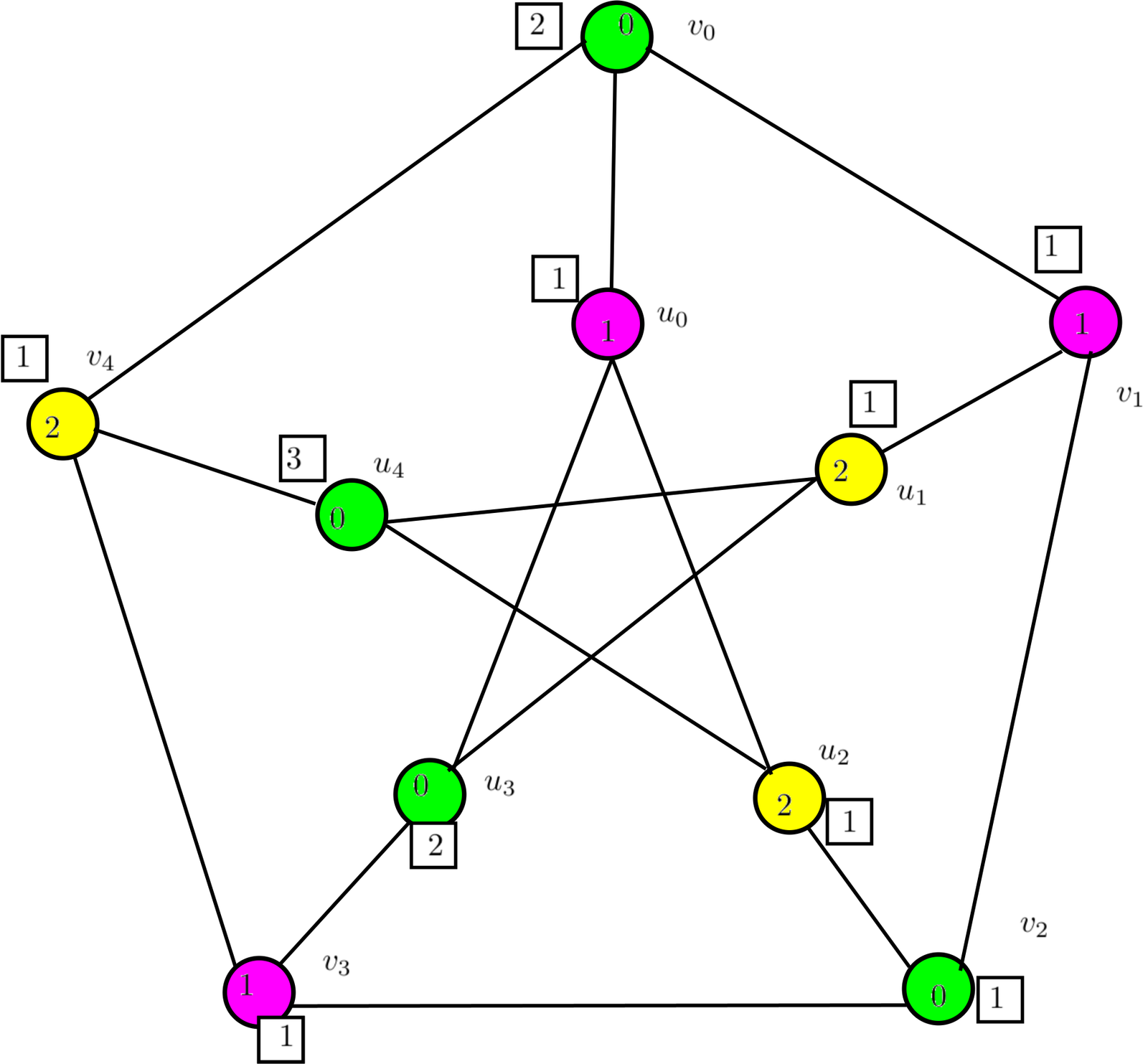
Figure 1 shows the Petersen graph \(P(5,2)\) together with a gap-\([3]\)-vertex labelling.
Watkins showed that \(P(n,k)\) is bipartite if and only if \(n\) is even and \(k\) is odd [6]. Since \(P(n,k)\) is connected and cubic, Brooks’ theorem gives the following chromatic-number description: \[ \chi(P(n,k))= \begin{cases} 2, & n \text{ is even and } k \text{ is odd},\\ 3, & \text{otherwise}. \end{cases}\tag{1}\]
The next elementary observation supplies the lower bound used throughout the paper.
Lemma 2.2. For every generalized Petersen graph \(P(n,k)\), \[\chi(P(n,k))\leq \chi_v^g(P(n,k)).\]
Proof. Suppose that \(P(n,k)\) admits a gap-\([q]\)-vertex labelling \(f\). Since the graph is cubic, every induced colour is a difference of two labels in \(\{1,\ldots,q\}\) and therefore belongs to \(\{0,1,\ldots,q-1\}\). Hence \(C_f\) is a proper colouring using at most \(q\) colours. Thus \(\chi(P(n,k))\leq q\). Minimizing over all admissible \(q\) gives the result. \(\square\)
For a gap-\([q]\)-vertex labelling \(f\) of \(P(n,k)\), the induced colours are \[ C_f(v_i)=\operatorname{MD}\{f(v_{i-1}),f(v_{i+1}),f(u_i)\},\tag{2}\] and \[ C_f(u_i)=\operatorname{MD}\{f(u_{i-k}),f(u_{i+k}),f(v_i)\}.\tag{3}\] The parameter classes treated below are summarized in Table 1. The classes are not intended to be disjoint.
| Conditions on \(P(n,k)\) | \(\chi_v^g(P(n,k))\) |
|---|---|
| \(n\) is even and \(k\) is odd | \(2\) |
| \(n\equiv 0\pmod{5}\), \(k\not\equiv 0\pmod{5}\), and \(P(n,k)\) is non-bipartite | \(3\) |
| \(n\equiv 0\pmod{4}\), \(n\geq 8\), and \(k\equiv 2\pmod{4}\) | \(3\) |
| \(n=2tk\), \(k\) is even, and \(t\geq 2\) | \(3\) |
| \(n\) is odd, \(n\geq 5\), and \(k=1\) | \(3\) |
| \(n\) is odd, \(n\geq 9\), \(n\not\equiv 0\pmod{5}\), and \(k=2\) | \(3\) |
| \(n=3k\) and \(k\geq 3\) | \(3\) |
Theorem 3.1. If \(n\) is even and \(k\) is odd, then \[\chi_v^g(P(n,k))=2.\]
Proof. Let \(G=P(n,k)\), where \(n\) is even and \(k\) is odd. Define \(f:V(G)\longrightarrow\{1,2\}\) by \[f(v_i)= \begin{cases} 1, & i \text{ even},\\ 2, & i \text{ odd}, \end{cases} \qquad f(u_i)=2 \quad (0\leq i\leq n-1).\] Because \(n\) is even, parity is well defined modulo \(n\). From (2), \[C_f(v_i)= \begin{cases} 0, & i \text{ even},\\ 1, & i \text{ odd}. \end{cases}\] Indeed, if \(i\) is even, the three neighbour labels of \(v_i\) are \(2,2,2\), whereas if \(i\) is odd they are \(1,1,2\).
Similarly, (3) gives \[C_f(u_i)= \begin{cases} 1, & i \text{ even},\\ 0, & i \text{ odd}. \end{cases}\] For an outer edge \(v_iv_{i+1}\), the endpoints have opposite parity and hence distinct induced colours. For every spoke \(v_iu_i\), the two displayed colour formulas are complementary. Finally, because \(k\) is odd, \(i\) and \(i+k\) have opposite parity, so \(C_f(u_i)\neq C_f(u_{i+k})\) on every inner edge. Hence \(C_f\) is proper, and therefore \(\chi_v^g(G)\leq2\).
By (1) and Lemma 2.2, \[2=\chi(G)\leq\chi_v^g(G).\] Consequently, \(\chi_v^g(P(n,k))=2\). \(\square\)
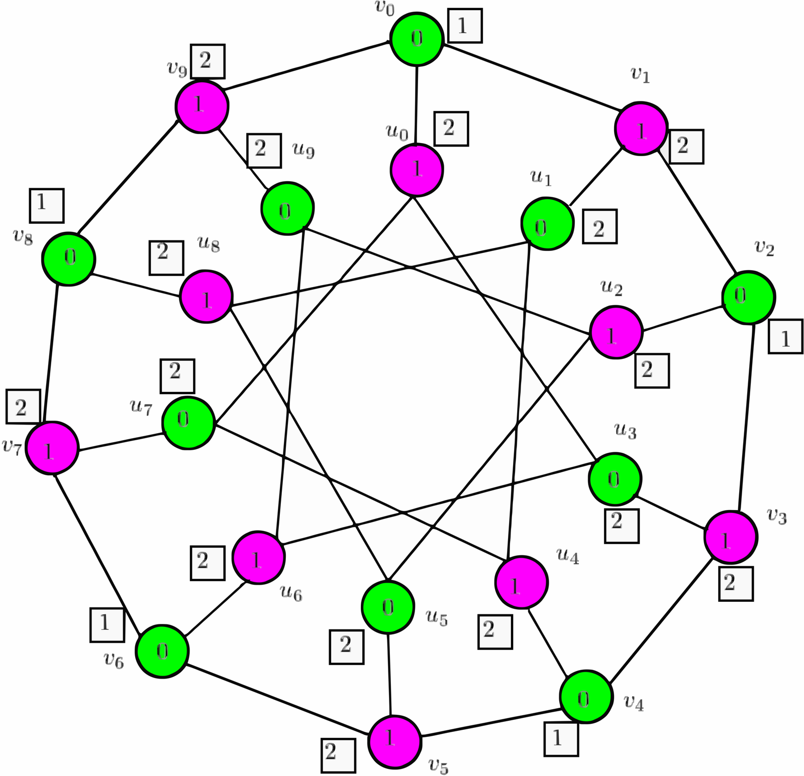
Figure 2 illustrates Theorem 3.1 for \(P(10,3)\).
As an immediate consequence, Theorem 3.1 gives the complete gap-\([2]\) classification within the generalized Petersen family.
Corollary 3.2. A generalized Petersen graph \(P(n,k)\) admits a gap-\([2]\)-vertex labelling if and only if \(n\) is even and \(k\) is odd.
Proof. The forward implication follows from Lemma 2.2: a non-bipartite generalized Petersen graph has chromatic number \(3\) by (1), and therefore cannot have vertex-gap number \(2\). The reverse implication is Theorem 3.1. \(\square\)
Theorem 3.3. Suppose that \[n\equiv0\pmod5, \qquad k\not\equiv0\pmod5,\] and that \(P(n,k)\) is non-bipartite. Then \[\chi_v^g(P(n,k))=3.\]
Proof. Let \(G=P(n,k)\). Define a gap-\([3]\)-vertex labelling by \[f(v_i)= \begin{cases} 2, & i\equiv0\pmod5,\\ 1, & \text{otherwise}, \end{cases} \qquad f(u_i)= \begin{cases} 3, & i\equiv4\pmod5,\\ 2, & i\equiv3\pmod5,\\ 1, & i\equiv0,1,2\pmod5. \end{cases}\] Since \(n\equiv0\pmod5\), these patterns close consistently around the graph. From (2), \[\begin{array}{c|ccccc} i\pmod5 & 0&1&2&3&4\\ \hline C_f(v_i)&0&1&0&1&2 \end{array}\] For the inner vertices there are two cases. If \(k\equiv\pm2\pmod5\), then \[\begin{array}{c|ccccc} i\pmod5 & 0&1&2&3&4\\ \hline C_f(u_i)&1&2&2&0&0, \end{array}\] whereas if \(k\equiv\pm1\pmod5\), then \[\begin{array}{c|ccccc} i\pmod5 & 0&1&2&3&4\\ \hline C_f(u_i)&2&0&1&2&1. \end{array}\] Consecutive entries in the \(v\)-row are distinct, so every outer edge is properly coloured. Comparing the \(v\)-row with either \(u\)-row componentwise shows that every spoke is properly coloured. Finally, shifting the appropriate \(u\)-row by \(\pm k\) modulo \(5\) gives a different value in every position, so every inner edge is properly coloured. Hence \(f\) is a gap-\([3]\)-vertex labelling and \(\chi_v^g(G)\leq3\).
By hypothesis \(G\) is non-bipartite, so (1) and Lemma 2.2 give \(\chi_v^g(G)\geq3\). Therefore \(\chi_v^g(P(n,k))=3\). \(\square\)
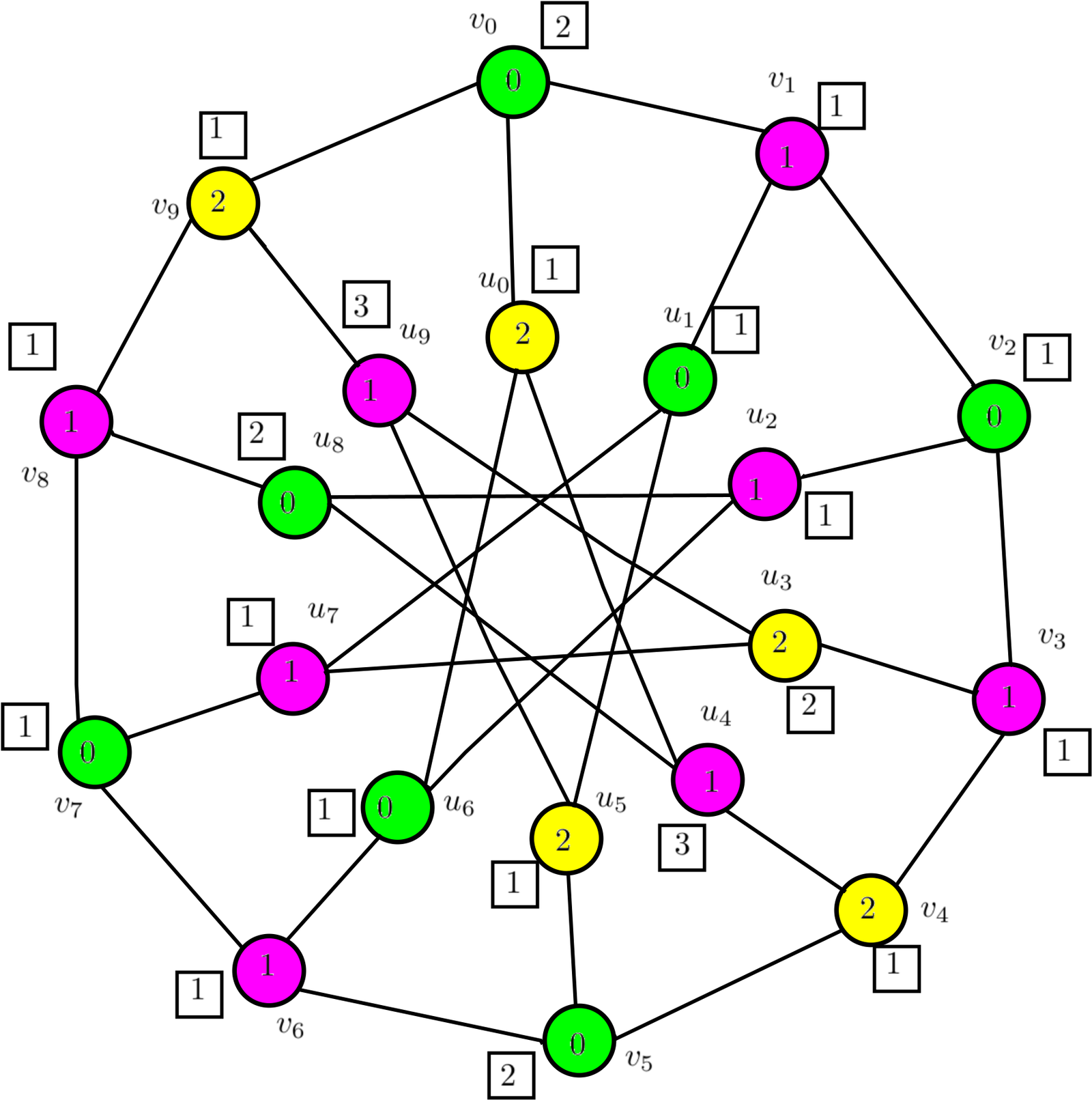
Figure 3 illustrates Theorem 3.3 for \(P(10,4)\).
Theorem 3.4. If \(n\equiv0\pmod4\), \(n\geq8\), and \(k\equiv2\pmod4\), then \[\chi_v^g(P(n,k))=3.\]
Proof. Let \(G=P(n,k)\) and define \[f(v_i)= \begin{cases} 2, & i=0,\\ 3, & i\equiv2\pmod4,\\ 1, & \text{otherwise}, \end{cases} \qquad f(u_i)= \begin{cases} 2, & i\equiv0,1\pmod4 \text{ and } i\neq0,\\ 1, & \text{otherwise}. \end{cases}\] A direct evaluation of (2) gives \[C_f(v_i)= \begin{cases} 0, & i=0 \text{ or } i\equiv2\pmod4,\\ 1, & i=1 \text{ or } (i\equiv0\pmod4 \text{ and } i\neq0),\\ 2, & \text{otherwise}. \end{cases}\] Similarly, \[C_f(u_i)= \begin{cases} 2, & i\in\{k,n-k\},\\ 0, & i\neq0 \text{ and } i\equiv0,1\pmod4,\\ 1, & \text{otherwise}. \end{cases}\] For outer edges, the displayed \(v\)-pattern gives distinct colours at consecutive indices. For spokes, the two displayed formulas are different at every index: the exceptional values \(i=0,1,k,n-k\) are covered explicitly, while the remaining indices follow immediately from their residue classes modulo \(4\).
It remains to consider an inner edge \(u_iu_{i+k}\). Since \(k\equiv2\pmod4\), adding \(k\) interchanges the residue classes \(0\leftrightarrow2\) and \(1\leftrightarrow3\) modulo \(4\). Thus a colour \(0\) is paired with \(1\) or \(2\), and a colour \(1\) is paired with \(0\) or \(2\). The only colour-\(2\) vertices are \(u_k\) and \(u_{n-k}\); each is adjacent through an inner edge to \(u_0\), of colour \(1\), and to a nonzero vertex with residue \(0\) modulo \(4\), of colour \(0\). Hence every inner edge is properly coloured. Therefore \(\chi_v^g(G)\leq3\).
Here \(n\) and \(k\) are both even, so \(G\) is non-bipartite. By (1) and Lemma 2.2, \(\chi_v^g(G)\geq3\). The result follows. \(\square\)
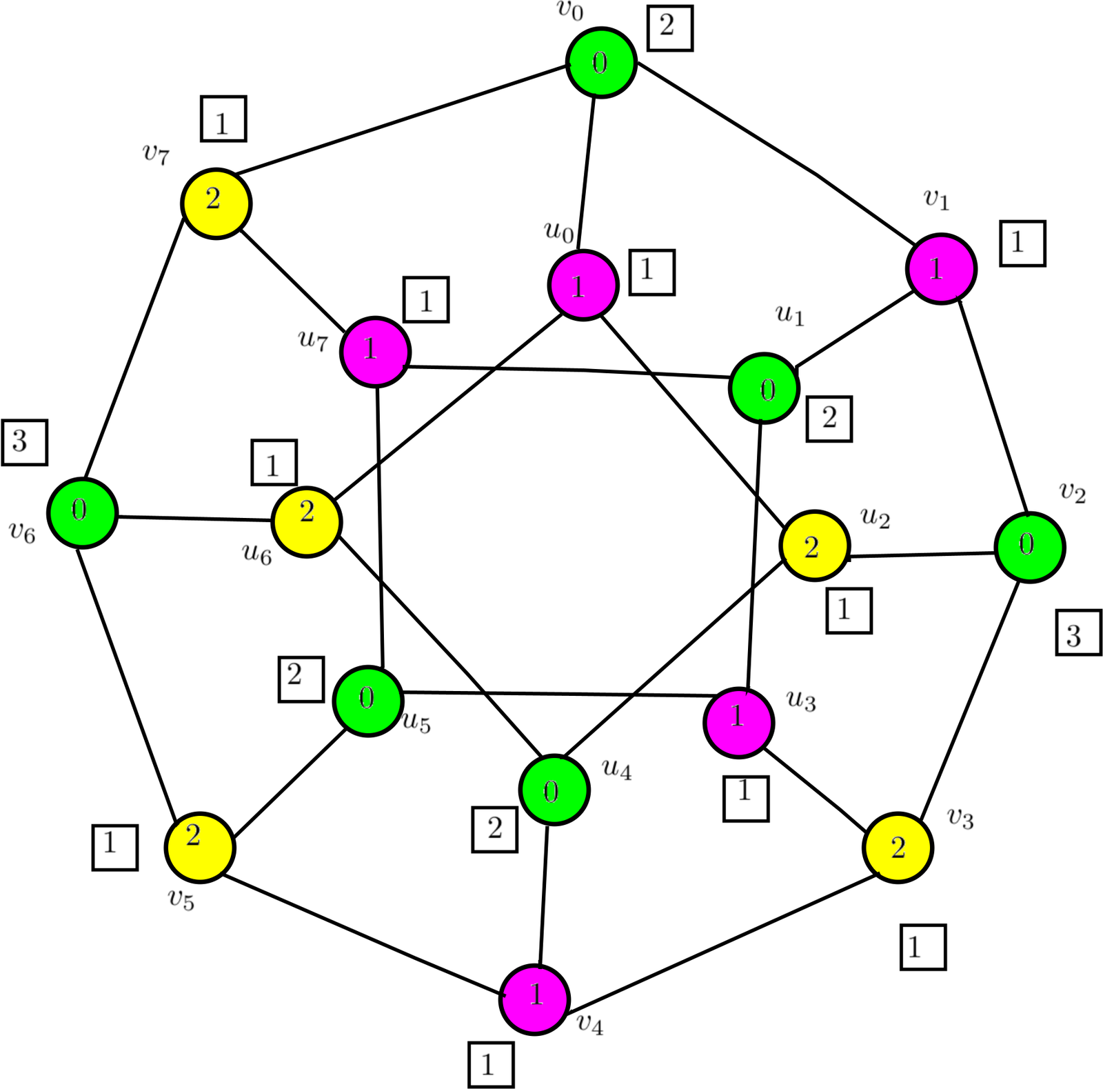
Figure 4 illustrates Theorem 3.4 for \(P(8,2)\).
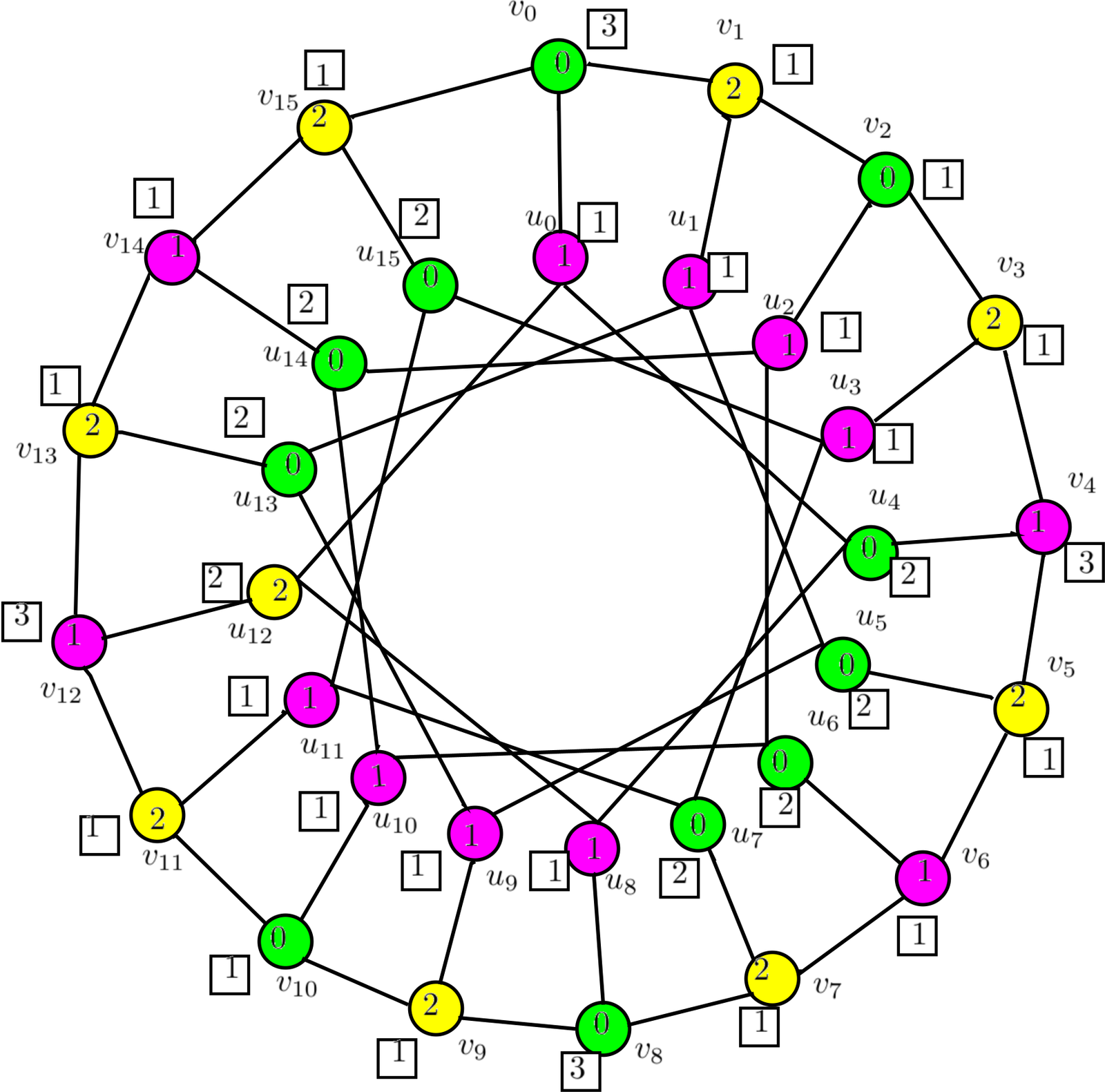
Theorem 3.5. Let \(n=2tk\), where \(k\) is even and \(t\geq2\). Then \[\chi_v^g(P(n,k))=3.\]
Proof. Let \(G=P(n,k)\). Partition the indices \(0,1,\ldots,n-1\) into the \(2t\) consecutive blocks \[B_j=\{jk,jk+1,\ldots,(j+1)k-1\}, \qquad 0\leq j\leq2t-1.\] Define \[f(v_i)= \begin{cases} 3, & i\equiv0\pmod4,\\ 1, & \text{otherwise}, \end{cases}\] and \[f(u_i)= \begin{cases} 1, & i\in B_j \text{ with } j \text{ even},\\ 2, & i\in B_j \text{ with } j \text{ odd}. \end{cases}\] Because \(k\) is even, adding or subtracting \(k\) moves an index from \(B_j\) to a block of opposite parity.
If \(i\) is odd, exactly one of \(i-1\) and \(i+1\) is divisible by \(4\). Hence the two outer-neighbour labels of \(v_i\) are \(1\) and \(3\), so \[C_f(v_i)=2.\] If \(i\) is even, both outer-neighbour labels are \(1\), and therefore \[C_f(v_i)= \begin{cases} 0, & i\in B_j \text{ with } j \text{ even},\\ 1, & i\in B_j \text{ with } j \text{ odd}. \end{cases}\] For \(u_i\), both inner neighbours lie in blocks of parity opposite to that of the block containing \(i\). Consequently, \[C_f(u_i)= \begin{cases} 1, & i\in B_j \text{ with } j \text{ even},\\ 2, & i\in B_j \text{ with } j \text{ odd and } i\equiv0\pmod4,\\ 0, & i\in B_j \text{ with } j \text{ odd and } i\not\equiv0\pmod4. \end{cases}\] Now every outer edge has one odd endpoint, of colour \(2\), and one even endpoint, of colour \(0\) or \(1\). On a spoke, an odd \(v_i\) has colour \(2\), while \(u_i\) has colour \(0\) or \(1\); if \(i\) is even, the displayed formulas again give distinct colours. Finally, the endpoints of every inner edge belong to blocks of opposite parity: a \(u\)-vertex in an even block has colour \(1\), while its inner neighbour in an odd block has colour \(0\) or \(2\). Hence \(C_f\) is proper and \(\chi_v^g(G)\leq3\).
Since \(n\) and \(k\) are even, \(G\) is non-bipartite. The lower bound \(\chi_v^g(G)\geq3\) follows from (1) and Lemma 2.2. Thus \(\chi_v^g(P(n,k))=3\). \(\square\)
Figure 5 illustrates Theorem 3.5 for \(P(16,4)\).
Theorem 3.6. If \(n\geq5\) is odd and \(k=1\), then \[\chi_v^g(P(n,1))=3.\]
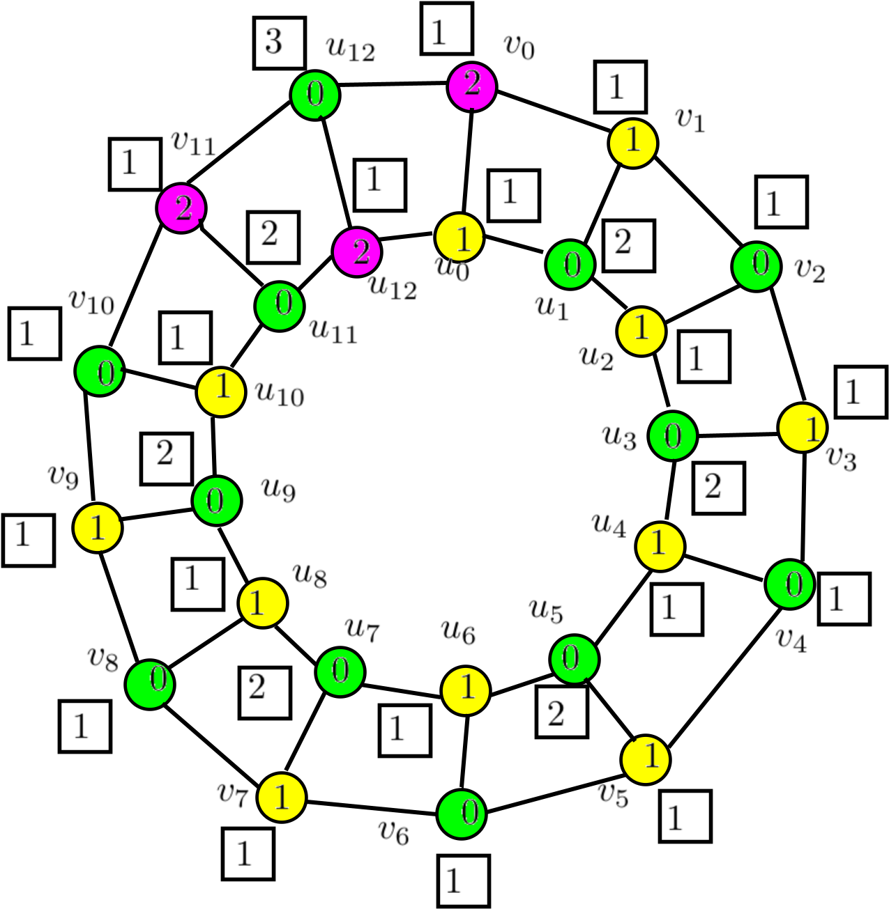
Proof. Let \(G=P(n,1)\) with \(n\) odd. Define \[f(v_i)= \begin{cases} 3, & i=n-1,\\ 1, & 0\leq i\leq n-2, \end{cases} \qquad f(u_i)= \begin{cases} 1, & i \text{ even},\\ 2, & i \text{ odd}. \end{cases}\] Using (2), \[C_f(v_i)= \begin{cases} 2, & i\in\{0,n-2\},\\ 0, & i \text{ even and } i\neq0,\\ 1, & i \text{ odd and } i\neq n-2. \end{cases}\] Using (3) with \(k=1\), \[C_f(u_i)= \begin{cases} 2, & i=n-1,\\ 1, & i \text{ even and } i\neq n-1,\\ 0, & i \text{ odd}. \end{cases}\] The outer colours alternate between \(0\) and \(1\) except at the two boundary vertices \(v_0\) and \(v_{n-2}\), both of which have colour \(2\); the wrap-around edge \(v_{n-1}v_0\) has colours \(0\) and \(2\). Hence every outer edge is proper. The two displayed formulas also show immediately that \(C_f(v_i)\neq C_f(u_i)\) for every spoke. Finally, along the inner cycle the colours alternate between \(1\) and \(0\), with the single boundary value \(C_f(u_{n-1})=2\), so every inner edge is proper. Therefore \(\chi_v^g(G)\leq3\).
Because \(n\) is odd, \(G\) is non-bipartite. The lower bound \(\chi_v^g(G)\geq3\) follows from Lemma 2.2, and the result follows. \(\square\)
Figure 6 illustrates Theorem 3.6 for \(P(13,1)\).
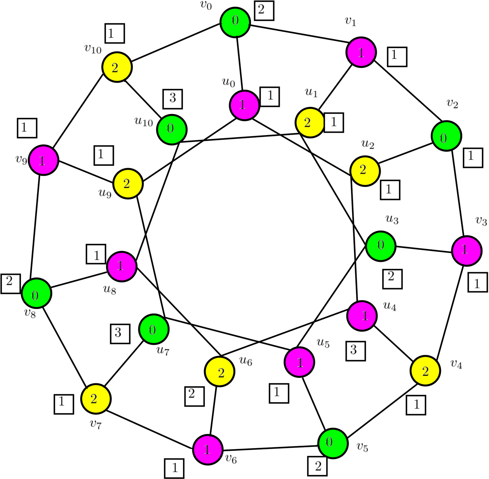
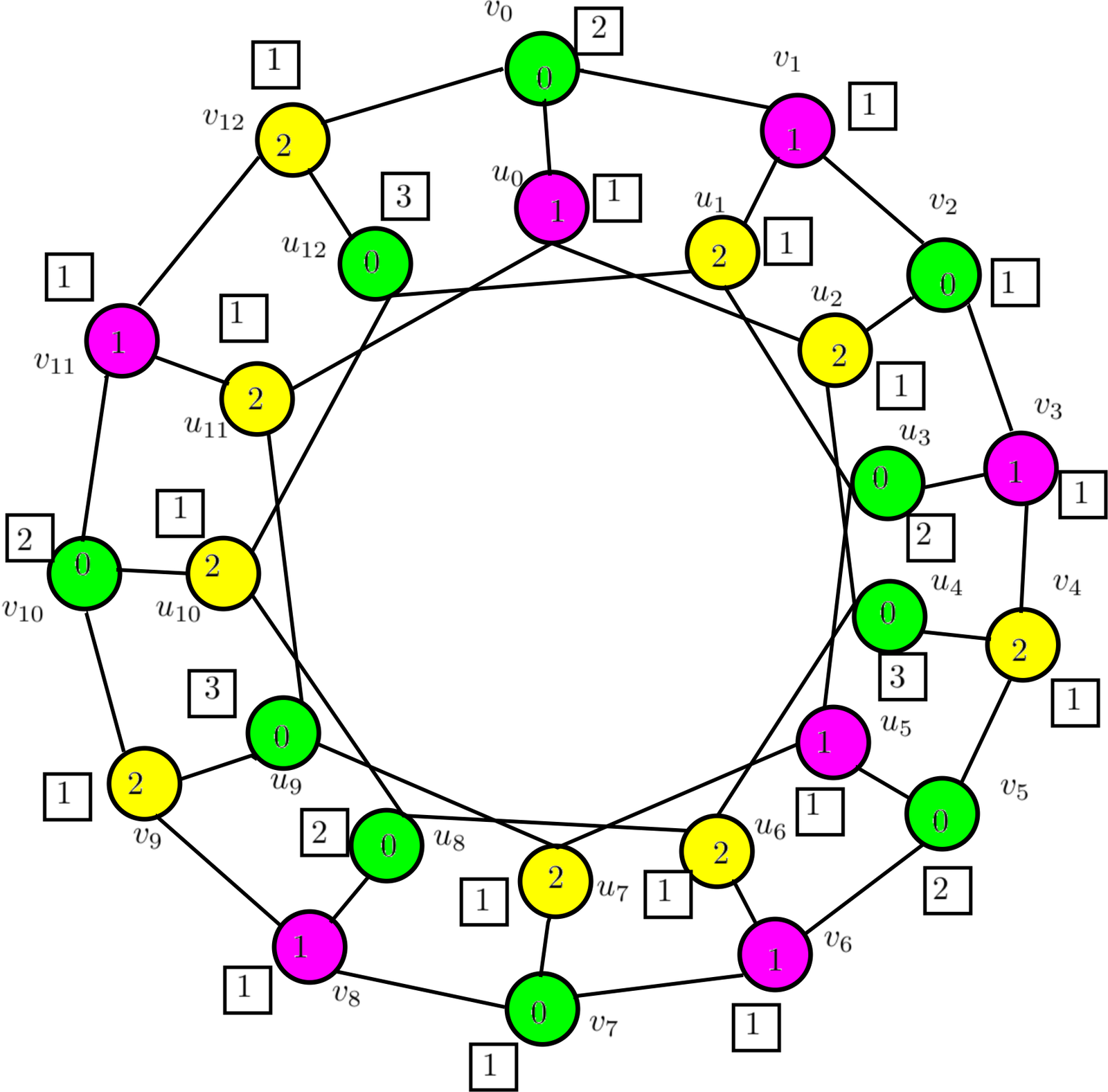
Theorem 3.7. Let \(n\geq9\) be odd, let \(n\not\equiv0\pmod5\), and let \(k=2\). Then \[\chi_v^g(P(n,2))=3.\]
Proof. Since \(n\) is odd and not divisible by \(5\), we have \[n\equiv1,3,7,\text{ or }9\pmod{10}.\] We give one explicit gap-\([3]\)-vertex labelling for each residue class. In Table 2, every index not listed in the corresponding row receives label \(1\). Congruence conditions are understood modulo \(5\).
| \(n\pmod{10}\) | \(\{i:f(v_i)=2\}\) | \(\{i:f(v_i)=3\}\) | \(\{i:f(u_i)=2\}\) | \(\{i:f(u_i)=3\}\) |
|---|---|---|---|---|
| \(1\) | \(\{i:i\equiv0\ (5),\ i\neq n-1\}\cup\{n-3\}\) | \(\varnothing\) | \(\{i:i\equiv3\ (5),\ i\neq n-3\}\cup\{n-5\}\) | \(\{i:i\equiv4\ (5),\ i\neq n-2\}\cup\{n-4,n-1\}\) |
| \(3\) | \(\{i:i\equiv0\ (5)\}\) | \(\varnothing\) | \(\{i:i\equiv3\ (5)\}\) | \(\{i:i\equiv4\ (5)\}\cup\{n-1\}\) |
| \(7\) | \(\{i:i\equiv0\ (5),\ i\neq n-2\}\) | \(\{n-2\}\) | \(\{i:i\equiv3\ (5)\}\cup\{n-1\}\) | \(\{i:i\equiv4\ (5)\}\cup\{1\}\) |
| \(9\) | \(\{i:i\equiv0\ (5),\ i\neq n-4\}\cup\{n-2\}\) | \(\varnothing\) | \(\{i:i\equiv4\ (5)\}\) | \(\{i:i\equiv3\ (5)\}\cup\{n-2\}\) |
For each row, substitute the labels from Table 2 into (2) and (3). The possible ordered colour pairs on the three types of edges are listed in Table 3. For compactness, \(ab\) denotes the ordered pair \((a,b)\).
| \(n\pmod{10}\) | \(v_iv_{i+1}\) | \(v_iu_i\) | \(u_iu_{i+2}\) |
|---|---|---|---|
| \(1\) | \(\{01,10,12,20\}\) | \(\{01,02,10,12,20,21\}\) | \(\{01,02,10,12,20,21\}\) |
| \(3\) | \(\{01,10,12,20\}\) | \(\{01,02,10,12,20\}\) | \(\{01,02,10,12,20,21\}\) |
| \(7\) | \(\{01,02,10,12,20\}\) | \(\{01,02,10,12,20,21\}\) | \(\{01,02,12,20,21\}\) |
| \(9\) | \(\{01,02,10,12,21\}\) | \(\{01,02,10,12,20,21\}\) | \(\{02,10,12,20,21\}\) |
No pair in Table 3 has equal entries. Hence the induced colouring is proper on every outer edge, every spoke and every inner edge. Thus, in all four residue classes, \(P(n,2)\) admits a gap-\([3]\)-vertex labelling and \(\chi_v^g(P(n,2))\leq3\).
Since \(n\) is odd, \(P(n,2)\) is non-bipartite. Therefore Lemma 2.2 gives the reverse inequality, and \(\chi_v^g(P(n,2))=3\). \(\square\)
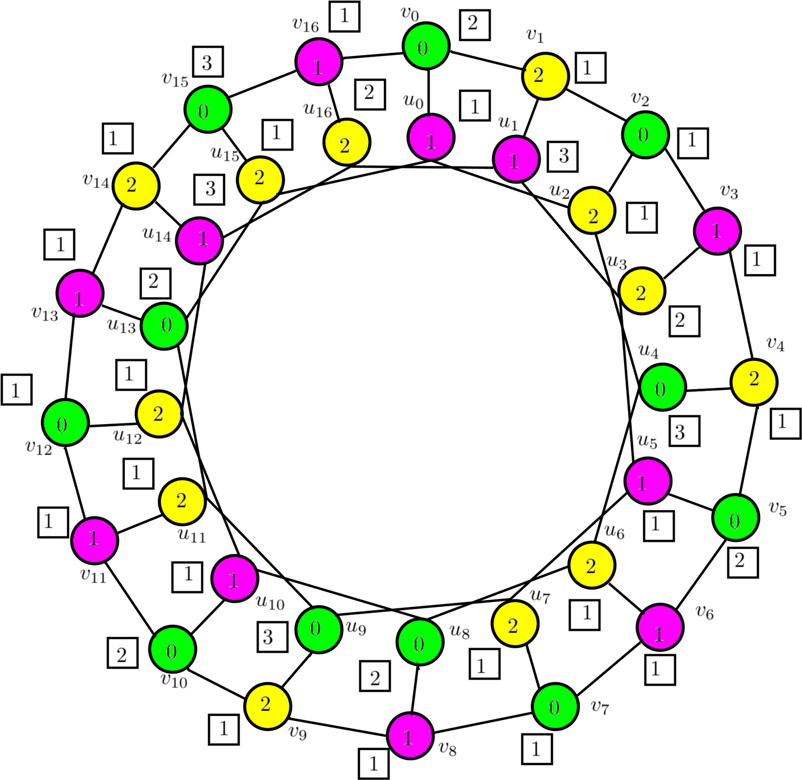
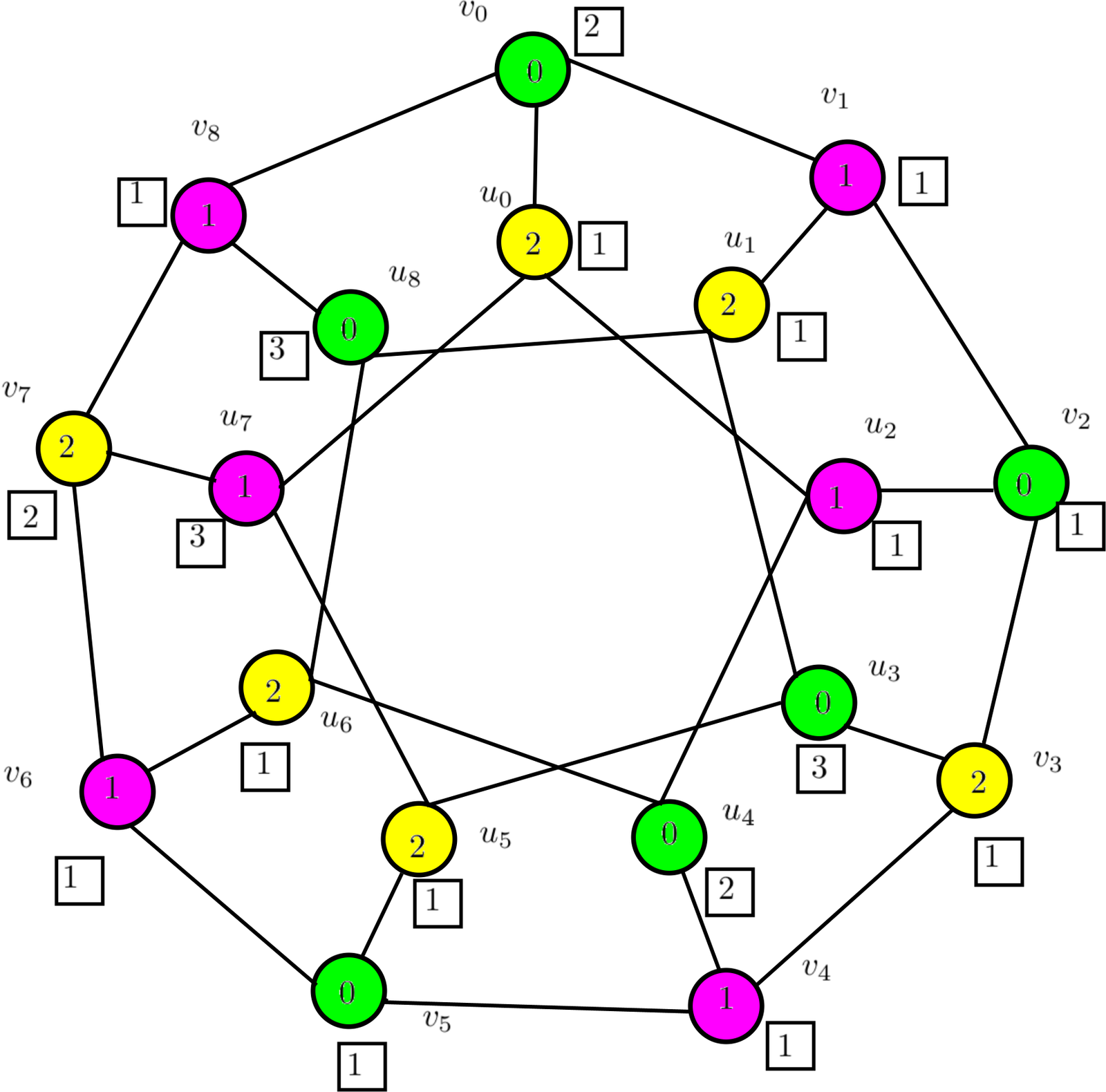
Figures 7, 8, 9, and 10 illustrate the four congruence classes in Theorem 3.7.
Theorem 3.8. If \(n=3k\) and \(k\geq3\), then \[\chi_v^g(P(n,k))=3.\]
Proof. Let \(G=P(3k,k)\). We distinguish the parity of \(k\).
Case 1: \(k\) is odd. Define \[f(v_i)= \begin{cases} 3, & i\geq k \text{ and } i \text{ is odd},\\ 1, & \text{otherwise}, \end{cases} \qquad f(u_i)= \begin{cases} 2, & 0\leq i\leq2k-2 \text{ and } i \text{ is even},\\ 1, & \text{otherwise}. \end{cases}\] Substitution into (2) and (3) shows that the possible induced-colour pairs on outer edges and spokes belong to \[\{(0,1),(1,0),(0,2),(2,0),(2,1)\},\] while the possible pairs on inner edges belong to \[\{(1,0),(0,2),(2,1)\}.\] Thus adjacent vertices always receive distinct induced colours.
Case 2: \(k\) is even. Define \[f(v_i)= \begin{cases} 2, & i\in\{0,k+3\},\\ 3, & i \text{ odd and } 3\leq i\leq k+1,\\ 3, & i \text{ even and } k+4\leq i\leq2k+2,\\ 1, & \text{otherwise}, \end{cases}\] and \[f(u_i)= \begin{cases} 2, & i=1,\\ 2, & i \text{ odd and } 2k+2<i\leq3k-1,\\ 2, & i \text{ even and } 4\leq i\leq k+2,\\ 1, & \text{otherwise}. \end{cases}\] Again, direct substitution into (2) and (3) shows that every ordered colour pair on an outer edge or a spoke belongs to \[\{(0,1),(1,0),(0,2),(2,0),(1,2),(2,1)\},\] and every ordered colour pair on an inner edge belongs to \[\{(1,0),(0,2),(2,1)\}.\] Hence \(C_f\) is proper in this case as well.
In either parity case, \(G\) admits a gap-\([3]\)-vertex labelling, so \(\chi_v^g(G)\leq3\). If \(k\) is odd, then \(n=3k\) is odd; if \(k\) is even, then both \(n\) and \(k\) are even. Thus \(G\) is non-bipartite in either case. By Lemma 2.2, \(\chi_v^g(G)\geq3\), and therefore \(\chi_v^g(P(3k,k))=3\). \(\square\)
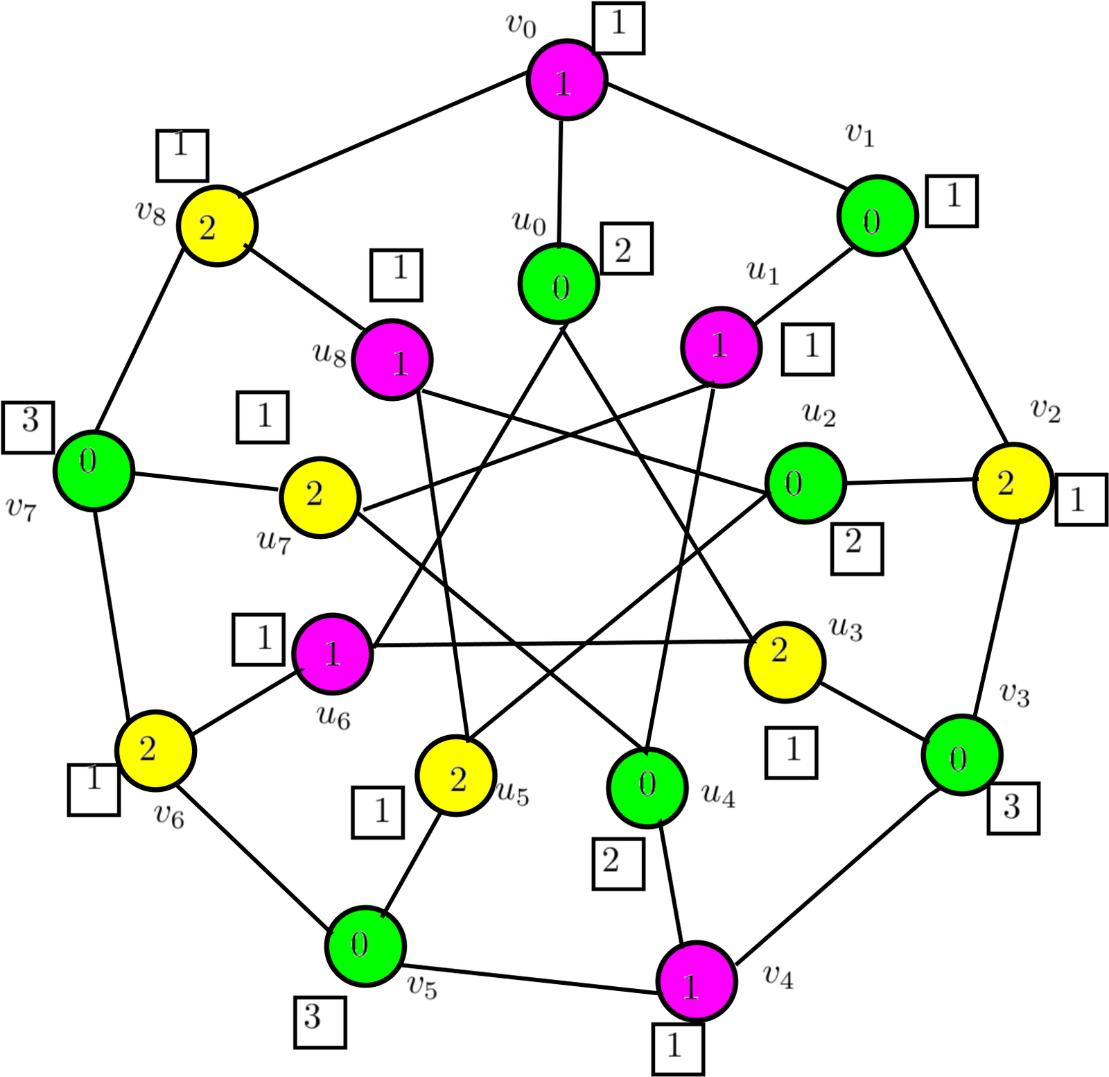
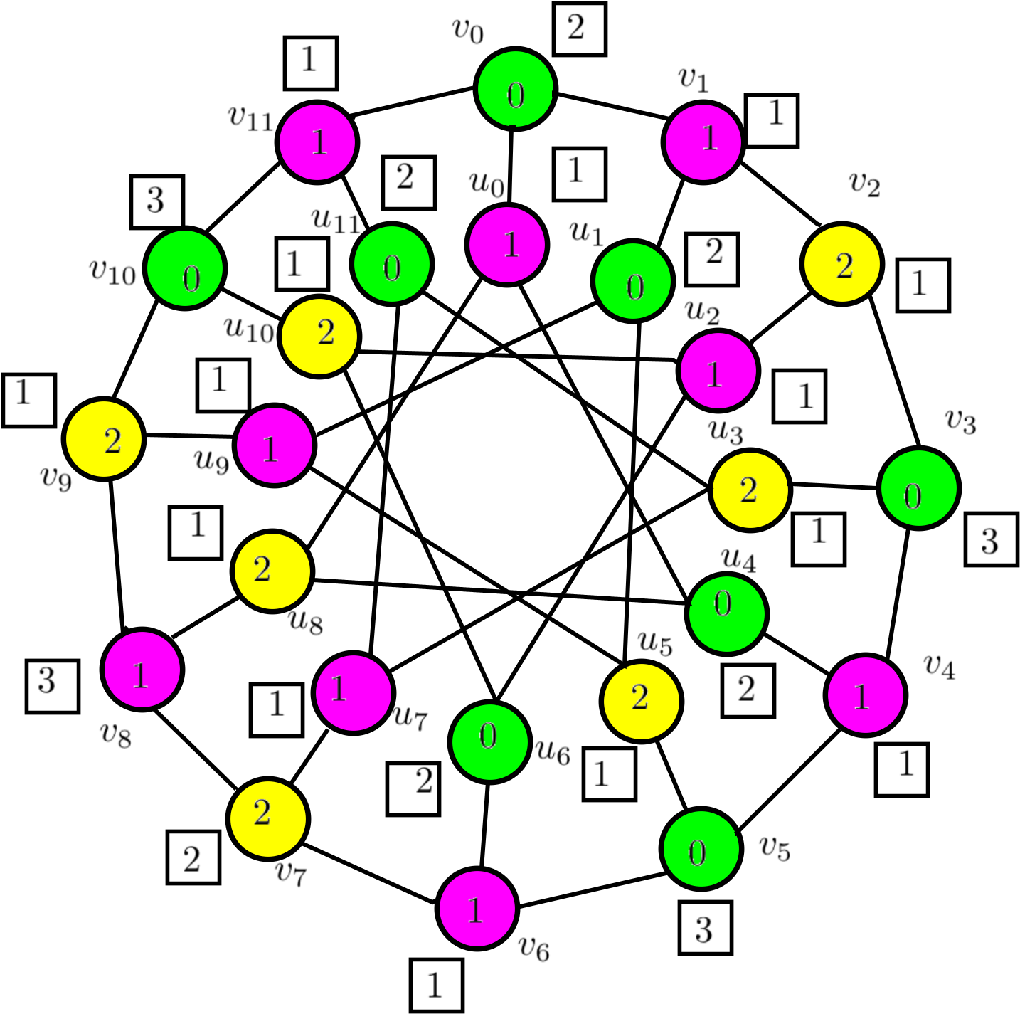
Figures 11 and 12 illustrate the two parity cases in Theorem 3.8.
The two smallest exceptional parameter pairs in the conjectural classification can be settled directly.
Proposition 3.9. The generalized Petersen graphs \(P(3,1)\) and \(P(6,2)\) satisfy \[\chi_v^g(P(3,1))=\chi_v^g(P(6,2))=4.\]
Proof. Both graphs are non-bipartite, so Lemma 2.2 gives \(\chi_v^g\geq3\). Since the graphs have only \(6\) and \(12\) vertices, respectively, the possibility \(q=3\) can be checked exhaustively: none of the \(3^6=729\) labellings of \(P(3,1)\) and none of the \(3^{12}=531441\) labellings of \(P(6,2)\) induces a proper colouring.
For the upper bound, order the labels as \[(f(v_0),\ldots,f(v_{n-1});f(u_0),\ldots,f(u_{n-1})).\] For \(P(3,1)\), the assignment \[(1,1,2;2,4,1)\] is a gap-\([4]\)-vertex labelling; its induced colours are \[(1,3,0;3,1,2).\] For \(P(6,2)\), the assignment \[(1,1,1,1,2,4;4,1,2,3,1,1)\] is a gap-\([4]\)-vertex labelling; its induced colours are \[(3,0,1,2,3,1;1,2,3,0,2,3).\] A direct check on the three edge types shows that adjacent vertices receive distinct induced colours in each case. Hence both vertex-gap numbers are \(4\). \(\square\)
We have determined the vertex-gap number for several broad classes of generalized Petersen graphs. Theorem 3.1 and Corollary 3.2 provide a complete characterization of the gap-\([2]\) case: \(\chi_v^g(P(n,k))=2\) exactly when \(P(n,k)\) is bipartite, equivalently when \(n\) is even and \(k\) is odd. For the non-bipartite families in Theorems 3.3–3.8, explicit gap-\([3]\)-vertex labellings show that the vertex-gap number equals the chromatic number, namely \(3\).
The remaining generalized Petersen graphs are not covered by the constructions above. Proposition 3.9 shows that the small graphs \(P(3,1)\) and \(P(6,2)\) are exceptional: their vertex-gap number is \(4\) although their chromatic number is \(3\). This motivates the following conjecture.
Conjecture 4.1. For every generalized Petersen graph \(P(n,k)\), \[\chi_v^g(P(n,k))= \begin{cases} 4, & (n,k)\in\{(3,1),(6,2)\},\\ 2, & n \text{ is even and } k \text{ is odd},\\ 3, & \text{otherwise}. \end{cases}\]
Establishing Conjecture 4.1 would complete the determination of the vertex-gap number for the entire generalized Petersen family. A natural next step is therefore to develop constructions that cover the remaining non-bipartite parameter pairs, or to identify additional exceptional graphs if they exist.
The authors declare that they have no conflicts of interest related to this work.
This research received no external funding.
This study is theoretical and does not involve the generation or analysis of datasets; therefore, data availability is not applicable.
All authors contributed equally to the conception, development, and preparation of this manuscript. All authors have read and approved the final version of the manuscript for publication.