
In the field of home surveying, airborne LiDAR technology has recently grown in importance. A type of laser detection and ranging system known as airborne LIDAR combines laser ranging, GPS, an inertial navigation system (INS), and a CCD camera mounted on fixed-wing aircraft or helicopters [1]. It has a high degree of accuracy and is capable of acquiring three-dimensional spatial data of the terrain surface in real time [2,3]. However, it is very difficult to conduct mapping operations with LIDAR equipment on board aeroplanes in terms of time and money due to the restrictions of aviation control and flight conditions. Small in size and light in weight, lightweight LIDAR lowers the technical bar for airborne LIDAR while reducing data acquisition costs. It is suitable for mounting on delta-wing or unmanned aerial vehicles with low altitude flight, simple takeoff conditions, and minimal aviation control. This technology has been widely applied to the creation of urban 3D models, the extraction of urban roads, and the acquisition of DigitalTerrain Models (DTM) [4,5]. For 3D modelling and the extraction of urban roads, automatic point cloud classification is crucial [6,7]. Two categories of automatic point cloud categorization techniques are currently available: the first uses geometric restrictions to categorise point clouds, while the second uses machine learning.
Multiple constraints must be set in the first geometric constraint-based point cloud classification approach in order to categorise each category. The road network is first segmented using the region growth law and the different characteristics of the various categories, and [8,9] manually extracts the seed points containing elevation information and reflection intensity information. The road network is then refined and denoised to obtain a road network with redundant roads and noise removed. According to the notion of greatest inter-class variance, the ground and non-ground point patches are split in [10,11], and the non-ground classes are divided into buildings, vegetation, etc. depending on a number of criteria. Three binary classifiers are employed in [12] to categorise the water bodies, gravel, bedrock, and flora in point cloud data of nature settings. The corn is recognised by integrating it with the remote sensing image in [13,14], and the feature points are then separated using Axelsson’s modified asymptotic triangular mesh by removing the medium-height vegetation points.
In the second machine-learning-based method for categorising point clouds, [15] built various feature vectors, merged the colour data to divide the point cloud into multiple scales, and then used Random Forest (RF) to divide the point cloud into six groups. According to the regularity of the feature distribution, a Bayesian model is presented in [16], and the discriminant rule based on the JointBoost classifier is enhanced by applying contextualization, which decreases the dimension of the feature vectors and the classification time. In [17], the point cloud data is clustered using the surface growth method, the feature vectors are built face to face, and the point cloud is classified using the Support Vector Machine (SVM), which has a higher level of classification accuracy because the clustered point cloud data contains more semantic information. In [18], multiple scales are set up, the dimensional features of the features are calculated at each scale, and the features are classified by SVM to find the best combination of scales, realising the classification of point cloud through the hyperplane’s best differentiation effect. Multiple scale features are extracted from the point cloud data and used as the local features of the points in [19] to address the issue that the PointNet algorithm is weak in describing the local features of the point cloud. After combining the local features with the extracted global features, the PointNet algorithm is then used for classification. Studies reveal that this approach outperforms other neural network methods in terms of classification accuracy.
Although the aforementioned techniques can produce classifications with a high degree of accuracy, significant issues remain. As an illustration, the raster grid classification method must be converted from the geometric constraints classification method, and elevation conversion requires elevation interpolation, which introduces errors. Additionally, a single LiDAR data source may be affected by issues like feature occlusion and data noise, thus, more sophisticated data processing techniques are required to increase the precision and stability of measurements; When classifying point clouds with multiple binary classifiers, cumulative errors are more likely to occur; however, feature vector redundancy is simple to achieve when classifying point clouds with machine learning algorithms. It is simple to produce cumulative errors when classifying point clouds with numerous binary classifiers; when employing machine learning methods, it is simple to experience the feature vector redundancy phenomena, which results in lengthy classification times or even overfitting issues [20].
This work suggests an airborne LiDAR point cloud classification approach based on the fusing of several base eigenvectors to address the aforementioned issues. This method can increase the classification accuracy by supplying additional semantic information for point cloud classification. This paper considers using this technology to measure house corners in rural cadastral surveys in order to decrease the workload of the field measurement of house corners and improve work efficiency. The lightweight LIDAR carried by delta wings is characterised by high precision and easy flight conditions. Beidachu Village in Beidachu Township of Yanqi County was chosen as the test object to clarify the technical process, efficiency, and accuracy of light airborne LIDAR applied to rural residential housing survey, and the light LIDAR carried out ultra-low-altitude, high-density, and high-overlap data collection by delta-wing in order to fully grasp the operational process of light airborne LIDAR [21], to clarify its planimetric accuracy and constraints, and to determine.
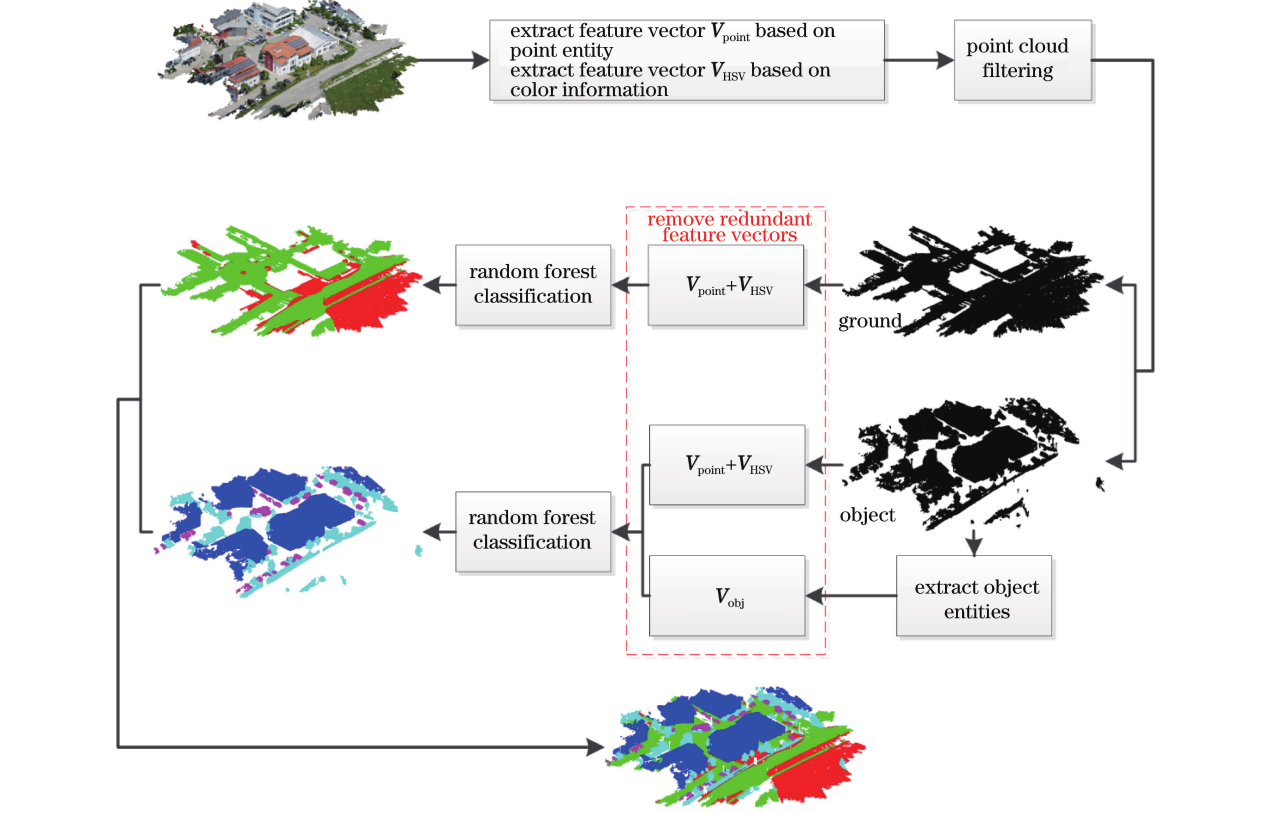
Figure 1 depicts the flow chart for the classification technique used in this paper. The method extracts point primitive feature vectors and colour information feature vectors in that order. The point primitive feature vectors include 3- and 7-dimensional feature vectors that were extracted using surface information as well as eigenvalue- and elevation-based 7-dimensional feature vectors. 6-dimensional extracted feature vectors make up the feature vector for colour information. The data is filtered, the feature points and ground points are separated, and then the ground points and feature points are classified independently using the recovered feature vectors. The ground points are classified by combining the extracted feature vectors with the colour information feature vectors, while the feature points are classified by extracting 8-dimensional feature vectors based on the objects after obtaining the object primitives . In order to improve the classification accuracy, the redundant vectors need to be removed in the final stage.
Specifically, it includes the following steps:
point primitive feature vector extraction;
color information feature vector extraction;
object primitive acquisition based on density clustering;
object primitive feature vector extraction;
redundant feature vector removal based on FSRF.
By statistically analysing the neighbouring points in the point cloud, it is possible to determine the geometric properties of the LiDAR point cloud, which can be used to successfully discern things like plants, buildings, and automobiles. The point cloud neighbourhood can be specified in one of three ways:
k-neighborhood, or the neighbourhood made up of the k closest points to the current judgement point;
sphere neighbourhood, or the neighbourhood made up of points with a radius of less than r from the current judgement point; and
cylinder neighbourhood, or the neighbourhood made up of points contained in a cylinder with the current judgement point at the centre [22].
The neighbourhood information of the point cloud is obtained in this study using the k-neighborhood definition method. The k-neighborhood definition approach is more effective than the other two methods and is appropriate for classifying huge amounts of point cloud data. Due to the homogeneous density of the point cloud data produced by airborne LiDAR, the k-neighborhood definition method can reliably extract the geometric features of the point. Eigenvalue-based, elevation-based, and surface-based eigenvectors are among the eigenvectors based on point primitives.
The local 3D structure of the point cloud, as well as its unique geometric qualities, can be described by the eigenvectors built using the eigenvalues. They can also be used to differentiate between different kinds of point clouds. This paper extracts three eigenvectors, Linearity, Planarity, and Scatter, to represent the linear, planar, and three-dimensional structures of local point clouds, respectively, and adds Anisotropy, Eigenentropy, and Omnivariance to take advantage of the differences in the 3D structure of point clouds among various categories. To describe the geometric properties of the point cloud, the four feature vectors anisotropy, eigenentropy, omnivariance, and surfacevariation are introduced [23].
The neighbouring point covariance tensor is created by using the current judgement point as the centre and finding its nearest \(k\) points to form the neighbouring point set \(P = \left\{ {{{\bf{p}}_1},{{\bf{p}}_2}, \cdots ,{{\bf{p}}_i}, \cdots ,{{\bf{p}}_k}} \right\}\). The neighbouring point covariance tensor is then constructed as follows.
\[\label{e1} \mathbf{C}_{\mathrm{x}}=\frac{1}{k} \sum_{i=1}^k\left(\mathbf{p}_i-\hat{\mathbf{p}}\right)\left(\mathbf{p}_i-\hat{\mathbf{p}}\right)^{\mathrm{T}},\tag{1}\] where \(\widehat {\bf{p}}\) is the location of the centre of the \(k\) nearby points, calculated as
\[\label{e2} \widehat {\bf{p}} = {\operatorname{argmin} _p}\sum\limits_{i = 1}^k {\left\| {{{\bf{p}}_i} – \sum\limits_{i = 1}^k {{{\bf{p}}_i}} } \right\|} .\tag{2}\]
From the covariance tensor can be calculated to obtain its three eigenvalues \({\lambda _1} > {\lambda _2} > {\lambda _3} > 0\), which are normalized so that \({\lambda _1} + {\lambda _2} + {\lambda _3} = 1\), three eigenvalues can be constructed seven eigenvectors, as shown in Table 1.
| Eigenvector | Size |
|---|---|
| Linearity | \({V_1} = ({\lambda _1} – {\lambda _2})/{\lambda _1}\) |
| Planarity | \({V_2} = ({\lambda _2} – {\lambda _3})/{\lambda _1}\) |
| Scatter | \({V_3} = {\lambda _3}/{\lambda _1}\) |
| Anisotropy | \({V_4} = ({\lambda _1} – {\lambda _3})/{\lambda _1}\) |
| Eigenentropy | \({V_5} = – \sum\limits_{{i^\prime } – 1}^3 {{\lambda _{{i^\prime }}}} \times \ln \left( {{\lambda _{{i^\prime }}}} \right)\) |
| Omnivariance | \({V_6} = \root 3 \of {{\lambda _1} \times {\lambda _2} \times {\lambda _3}}\) |
| Surface variation | \({V_7} = {\lambda _3}\) |
Since distinct feature point clouds have quite varied elevation characteristics, the features’ types can be accurately determined by the elevation characteristics. For instance, the elevation distributions of the nearby points in various point clouds differ, as do the elevation kurtosis and elevation skewness of regular and irregular features. Additionally, the elevation of structures is typically higher than that of vegetation. The elevation characteristic vectors added in this paper are shown in Table 2, where Height above is the difference in elevation between the current point and the largest point in the neighbouring point set, Heightbelow is the difference in elevation between the current point and the smallest point in the neighbouring point set, and Heightaverage is the average value. This is done in order to take advantage of the differences in elevation characteristics between different categories. Heightaverage, \({z_p}\) is the elevation of the judgment point, \(z({p_i})\) is the elevation of the neighboring point, \({z_{\max }}({p_i})\) is the maximum value of the elevation in the set of neighboring points, \({z_{\min }}({p_i})\) is the minimum value of the elevation in the set of neighboring points.
| Eigenvector | Size |
|---|---|
| Height above | \({V_8} = {z_{\max }}\left( {{{\bf{p}}_i}} \right) – {z_{\text{p}}}\) |
| Height below | \({V_9} = {z_{\text{p}}} – {z_{\min }}\left( {{{\bf{p}}_i}} \right)\) |
| Height average | \({V_{10}} = \sum\limits_{i = 1}^k z \left( {{{\bf{p}}_i}} \right)/k\) |
| Vertical Range | \({V_{11}} = {z_{\max }}\left( {{{\bf{p}}_i}} \right) – {z_{\min }}\left( {{{\bf{p}}_i}} \right)\) |
| Height standard deviation | \({V_{12}} = \sqrt {\frac{1}{k}\sum\limits_{i = 1}^k {{{\left[ {z\left( {{{\bf{p}}_i}} \right) – {V_{10}}} \right]}^2}} }\) |
| Height kurtosis | \({V_{13}} = \frac{{\sum\limits_{i = 1}^k {{{\left[ {z\left( {{{\bf{p}}_i}} \right) – {V_{10}}} \right]}^3}} }}{{{{\left\{ {\sum\limits_{i = 1}^k {{{\left[ {z\left( {{{\bf{p}}_i}} \right) – {V_{10}}} \right]}^2}} } \right\}}^{\frac{3}{2}}}}}\) |
| Height skewness | \({V_{14}} = \frac{{\sum\limits_{i = 1}^k {{{\left[ {z\left( {{{\bf{p}}_i}} \right) – {V_{10}}} \right]}^4}} }}{{{{\left\{ {\sum\limits_{i = 1}^k {{{\left[ {z\left( {{{\bf{p}}_i}} \right) – {V_{10}}} \right]}^2}} } \right\}}^2} – 3}}\) |
This work integrates the colour information for classification in order to increase the classification accuracy of point clouds. The colour information of various sorts of elements varies greatly, for instance, highways are grayish-white and vegetation is either light green or dark green, making it easy to tell them apart. However, when collecting point cloud data, light is able to quickly modify the colour information [24]. This study converts the RGB colour space to HSV colour space because the HSV colour space can offer more information than the RGB colour space [5] and the extracted hue (H) information can lessen the impact of ambient light. Smith [13] first developed the HSV colour system, and the equation for translating the RGB colour space to the HSV colour space is The following formula will convert RGB to HSV colour space:
\[\label{e3} H=\left\{\begin{array}{cc} 0^{\circ}, & \Delta=0, \\ 60^{\circ} \times\left(\frac{G^{\prime}-B^{\prime}}{\Delta}+0\right), & C_{\max }=R, \\ 60^{\circ} \times\left(\frac{B^{\prime}-R^{\prime}}{\Delta}+2\right), & C_{\max }=G, \\ 60^{\circ} \times\left(\frac{R^{\prime}-G^{\prime}}{\Delta}+4\right), & C_{\max }=B, \end{array}\right.\tag{3}\]
\[\label{e4} S=\left\{\begin{array}{l} 0, \quad C_{\max }=0, \\ \frac{\Delta}{C_{\max }}, \quad C_{\max } \neq 0, \end{array}\right.\tag{4}\]
\[\label{e5} V = {C_{\max }},\tag{5}\] where \(H\) stands for hue, \(S\) for saturation, \(V\) for brightness, and \(R, G\), and \(B\) are the point cloud data’s values for the red, yellow, and blue colour channels;
\[\label{e6} \begin{cases} R^{\prime}=R / 255, \\ G^{\prime}=G / 255, \\ B^{\prime}=B / 255, \\ C_{\max }=\max \left(R^{\prime}, G^{\prime}, B^{\prime}\right), \\ C_{\min }=\min \left(R^{\prime}, G^{\prime}, B^{\prime}\right), \\ \Delta=C_{\max }-C_{\min }. \end{cases}\tag{6}\]
In this study, the neighbouring points-defined as those with a distance from the present judgement point of less than 3 meters-are the points whose HSV colour information and average HSV colour information are employed as feature vector inputs.
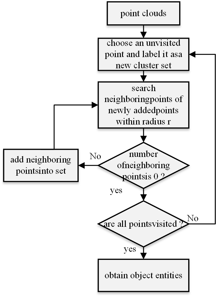
It is important to initially acquire the object primitives in order to extract the feature vectors based on the objects. This research uses a density-based approach to extract object primitives from a point cloud. The next phases are part of the algorithm flow for extracting object primitives, which is depicted in Figure 2, as following step:
Find an unvisited point in the point cloud.
Add the set of neighbouring points to the set of points if the number of neighbours is not zero; otherwise, repeat step 1 for the set of neighbouring points.
Iterate through the unvisited points, add new set labels, and carry out step 1 if the number of neighbouring points is 0.
Continue doing steps 1 through 3 until every point has been reached.
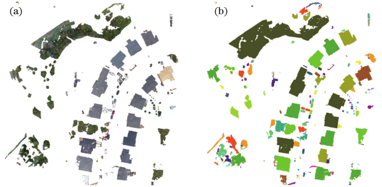
The schematic diagram for object primitive extraction is shown in Figure 3. Following the extraction of object primitives, Figure 3(a) displays the result seen in Figure 3(b). The colour of the feature points is displayed in Figure 3(b) in top view, and it can be seen that the point clouds of the various objects can be recognised clearly.
Each object is taken as the smallest unit after many object primitives have been extracted so that the points in each object have the same feature vector. The maximum height, minimum height, average height, and difference between the maximum height and minimum height of each object’s point cloud are extracted from this article and added to the feature vector set. The following methods are used to simultaneously extract the four properties of the object’s greatest surrounding rectangle and input them as eigenvectors [18].
Regular buildings can be distinguished from other irregular objects by looking at the ratio of the pixels on the xoy projected surface to the area of the greatest enclosing rectangle. Before determining the maximum enclosing rectangle, it is required to turn the point cloud data into 2D grid data by giving the grids containing point clouds a value of 1 and the grids without them a value of 0. The results of this point cloud rasterization using various grid sizes are shown in Figure 4. It is clear that the grid’s size significantly affects how the point cloud is rasterized. The rasterized shape is closer to the projected shape of the point cloud when the grid size is small, as illustrated in Figure 4(b), but the grid is denser. The shape of the rasterized shape differs from the projected shape of the point cloud when the size of the grid is big, as seen in Figure 4(c). The upper right corner of Figure 4(c) is gone, deviating from the geometry of the initial point cloud. Overall, point cloud rasterization produces jagged results, which is another feature of point cloud rasterization. The grid size of the point cloud rasterization in this study is set to 1m in order to combine the approximation of the point cloud rasterized shape and the processing effectiveness of the point cloud rasterization computation.
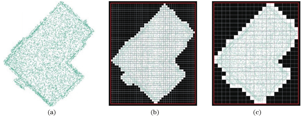
It is evident from Figure 4(a) that the predicted rectangularity will be incorrect if the building’s maximum enclosing rectangle is acquired directly. The largest encompassing rectangle box in this case has a lot of data gaps, thus it can’t accurately represent the building’s rectangular-like features. This paper first determines the direction of the building’s largest parallel side (as indicated by the dotted line in Figure 4(a)), then determines the angle between the parallel side’s vertical direction and the direction of the x-axis, and finally rotates the building by the angle shown in Figure 4(b) to reflect the building’s rectangularity. With this approach, it is simple to determine the length and width of the greatest enclosing rectangle because the length and width of the rotated building are parallel to the direction of the coordinate axis. Following rotation, each object’s length/width ratio \((L/W)\), volume of the largest enclosing box \((V')\), and area of the largest enclosing rectangle \((S')\) are retrieved and added to the set of feature vectors.
\[\label{e7} S^{\prime}=\left[\max \left(i_1\right)-\min \left(i_1\right)\right] \times\left[\max \left(j_1\right)-\min \left(j_1\right)\right] \times c_1,\tag{7}\] \[\label{e8} \begin{aligned} & \left\{\begin{array}{ll} L / W=\left[\max \left(j_1\right)-\min \left(j_1\right)\right] /\left[\max \left(i_1\right)-\min \left(i_1\right)\right], & j_1>i_1 \\ L / W=\left[\max \left(i_1\right)-\min \left(i_1\right)\right] /\left[\max \left(j_1\right)-\min \left(j_1\right)\right], & j_1 \leqslant i_1 \end{array}, V^{\prime}=S^{\prime} \times h_{\max },\right. \end{aligned}\tag{8}\] where \({i_1}\) is the row number of the 2D grid projected on the xoy plane; \({j_1}\) is the column number of the 2D grid projected on the xoy plane; \({c_1}\) is the spacing of the 2D grid projected on the xoy plane; and \({h_{\max }}\) is the maximum value of the object elevation.
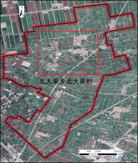
We selected Beidachu Village, a central and populous settlement in Beidachu Township, Yanqi County, which is situated in the plains, with a north-south corridor and flat terrain, as the test place for our experiment. The settlement contains a wide variety of homes, including multi-story buildings, earth dwellings, historic brick homes, new mixed-use homes, and old mixed-use homes, all of which serve as examples of various home types and are typical of rural residential land surveys. The test region, depicted as the black box in Figure 5, is within the aerial survey area, which has a total area of around \(5km^2\) [22].
This test used a 735kW power delta wing with a maximum load capacity of 250kg as the flight platform, carrying a lightweight airborne LIDAR with an integrated airborne LIDAR laser transmitter system, an aerial inertial navigation system, a camera, and a total weight of 13kg, with planar positioning accuracy of 10mm+110-6D and an elevation positioning accuracy of 20mm+110-6D.
The measurement accuracy of airborne LIDAR is mainly determined by the accuracy of eight measurements such as laser ranging \((S)\), GPS positioning \(\left( {{X_s},{Y_s},{Z_s}} \right)\), and IMU attitude and tracing angle (\(\theta\)). In the case of a certain measurement error of each parameter, the coefficients change with the scanning angle \(\theta\) and the ranging value \(S\). The scanning angle error is fixed and can be measured in the factory, so the coefficients change with the ranging value \(S\). The value of \(S\) is directly related to the altitude of flight, and the lower the altitude of flight, the smaller the value of \(S\) is, and the smaller the coefficients’ errors are. The lower the flight altitude, the smaller the \(S\) value, and the smaller the error of each coefficient. Considering the factors of flight safety, the flight altitude is set to 170m [].
In order to acquire the point cloud data, it was necessary to fly both horizontally and vertically in the direction of the house arrangement. To increase the point cloud density as much as possible, it was necessary to fly a low-altitude, high-overlap cross-course flight (see Table 3 for the technical parameters of airborne dimensional laser scanning data acquisition). This allowed for the complete acquisition of the houses’ texture information. The measuring area is just over 5 km2, consequently, there would be no need for more than one base station in the centre. It is important to turn on the GPS receiver 5 minutes before the delta wing lifts off and turn it off 5 minutes after the delta wing stops during flight operation in order to synchronise the observation with the GPS carried on the delta wing.
| Name | Parameter |
|---|---|
| Relative row height/m 1 | 75 |
| Flight speed/(km/h) | 110 |
| Laser emission frequency/kHz | 220 |
| Laser scanning angle/\(\theta\) | 75 |
| Laser bandwidth/m | 250 |
| Laser dot spacing/m | 0.15 |
In order to measure the coordinate system conversion, Xinjiang Bazhou CORS has covered the survey area. This ground control survey uses the network RIK method, measuring the ground control points while simultaneously recording the results of the WGS-84 and CGCS2000 coordinate systems.
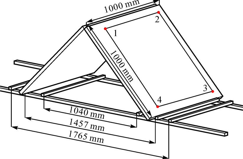
In order to ensure that the four measurement points were connected to the line formed by the closed 4-sided area of more than \(0.5m^2\), the distribution of the form shown in Figure 6 was used to measure the control markers in the deployment of the control panel. For the point cloud’s absolute accuracy adjustment, a total of 20 slopes were measured.
As checkpoints, a total of 36 house corner sites that were evenly spaced around the test area were measured. Some texture information is lost as a result of the sparse point cloud on the wall surface brought on by shading and occlusion, and the house corner points are not included in the point cloud. Out of 36 checkpoints, 30 house corner points are grabbed, for an 83.3% capture rate and a median error of 0.048 m. Table 4 displays the outcomes of the checking statistics.
| Maximum value/m | Min/m | Average value/m | Mean square error/m | Collection rate/(%) |
|---|---|---|---|---|
| 0.138 | 0.018 | 0.062 | 0.050 | 83.5 |
The measurement accuracy of the home corner points of the rural residential land survey is in accordance with the measurement accuracy of the boundary points in the “Cadastral Survey Procedure” (TD/T1001-2012), as stated in the Land Resources Development [2014] No. 101 document [24]. The outcomes of airborne LDAR point cloud vectorization of house corner points were analysed, and the statistical results are provided in Table 5 with reference to the precision index of boundary points in the “Cadastral Survey Regulations”.In this test, 83.3% of the house corner points were collected. Among them, 41.7% (14) of the house corner point errors are 5 cm, which can satisfy the “Cadastral Survey Regulations” requirements for the accuracy of the first level of boundary points, and 77.8% (28) of the house corner point errors are 10 cm, which can satisfy the “Cadastral Survey Regulations” requirements for the precision of the error in the first level of boundary points; For the precision of the error in the first level of boundary points, 83.3% (30) of the house corner points in the vectorized data can satisfy “Cadastral Survey Regulations,” and 83.3% (30) of the house corner points in the vectorized data can satisfy “Cadastral Survey Regulations” for the error in the first level of boundary points. The Cadastral Survey Regulations’ allowable error precision standards for level II boundary points can be met by all vectorized data, accounting for 83.3% (30) of the point location errors of house corner points.
| \(\leqslant\)5cm | \(\leqslant\)10cm | \(\leqslant\)15cm | Point cloud data not collected |
|---|---|---|---|
| 42.0 | 78.8 | 83.5 | 16.8 |
The point cloud data in this study is classified using Random Forest (RF), and the feature vectors are made up of three types of primitive feature vectors: point, object, and colour information. In this study, we use half of the test data as training data and half as test data. Fig. 7 illustrates the classification error rate using various combinations of feature vectors, including the single primitive and fused multi-subject feature vectors.
As demonstrated in Figure 7, the colour information feature vector set has the lowest classification error rate when the three single primitive feature vectors are utilised for classification, but the single primitive feature vector is unable to achieve this. However, utilising a single primitive feature vector will not result in the lowest classification error rate. The classification error rates of the three data sets are lower when multibasic feature vectors are merged than when utilising a single primitive feature vector. It is obvious that multikernel feature vector fusion classification accuracy is greater than single primitive feature vector classification accuracy.
The efficiency of the RF is examined in this research using comparative analysis using SVM and back propagation (BP) neural network. Recall (Re), precision (Pr), and F1 score are the evaluation indices, and Tables 6, 7 and 8 display the experimental findings.
Precision is a measure of the percentage of accurate classifications, while recall is a measure of categorization coverage. Recall and precision typically follow opposing trends in classification problems, so any rise in one will be accompanied by a fall in the other. As a result, the F1 score indication is added in this study as a reference for the previous two indicators [12].
| Category | Recall/% | Precision/% | F1 score | ||||||
|---|---|---|---|---|---|---|---|---|---|
| RF | SVM | BP | RF | SVM | BP | RF | SVM | BP | |
| Ground | 96.25 | 95.98 | 11.95 | 85.26 | 84.78 | 8.15 | 0.95 | 0.95 | 0.21 |
| High vegetation | 44.87 | 43.85 | 95.68 | 83.45 | 78.98 | 78.62 | 0.55 | 0.56 | 0.88 |
| Building | 97.85 | 97.50 | 0 | 81.56 | 79.99 | 0.1 | 0.88 | 0.87 | 0.45 |
| Road | 67.8 | 64.58 | 46.01 | 95.68 | 96.65 | 1.84 | 0.89 | 0.87 | 0 |
| Car | 60.68 | 52.04 | 92.85 | 50.26 | 58.20 | 49.81 | 0.56 | 0.56 | 0.65 |
| Human-made obiect | 21.28 | 48.65 | 16.65 | 41.20 | 39.56 | 36.01 | 0.26 | 0.24 | 0.07 |
| Mean | 64.58 | 61.60 | 34.52 | 72.56 | 73.63 | 30.14 | 0.56 | 0.63 | 0.28 |
| Category | Recall/% | Precision/% | F1 score | ||||||
|---|---|---|---|---|---|---|---|---|---|
| RF | SVM | BP | RF | SVM | BP | RF | SVM | BP | |
| Ground | 73.21 | 73.56 | 91.20 | 88.32 | 84.78 | 75.86 | 0.9 | 0.9 | 0.93 |
| High vegetation | 87.52 | 76.52 | 38.52 | 71.25 | 73.92 | 60.58 | 0.75 | 0.66 | 0.48 |
| Building | 91.88 | 77.50 | 2.05 | 71.56 | 73.59 | 60.32 | 0.78 | 0.77 | 0.45 |
| Road | 97.58 | 97.88 | 68.98 | 89.88 | 90.52 | 18.25 | 0.92 | 0.91 | 0.05 |
| Car | 50.98 | 7.15 | 30.25 | 54.85 | 60.21 | 18.89 | 0.96 | 0.94 | 0.25 |
| Human-made obiect | 50.28 | 0.1 | 0.1 | 13.05 | 0 | 0 | 0.52 | 0 | 0 |
| Mean | 67.78 | 58.72 | 38.52 | 68.52 | 66.32 | 42.52 | 0.66 | 0.58 | 0.35 |
| Category | Recall/% | Precision/% | F1 score | ||||||
| RF | SVM | BP | RF | SVM | BP | RF | SVM | BP | |
| Ground | 73.25 | 74.56 | 2.25 | 88.95 | 90.25 | 7.86 | 0.85 | 0.85 | 0.03 |
| High vegetation | 82.54 | 80.65 | 62.05 | 61.25 | 70.82 | 58.58 | 0.72 | 0.76 | 0.68 |
| Building | 82.88 | 87.50 | 65.268.56 | 70.58 | 59.32 | 0.74 | 0.75 | 0 | |
| Road | 77.5878.82 | 10.25 | 90.58 | 85.26 | 15.32 | 0.85 | 0.82 | 0.02 | |
| Car | 7.78063.52 | 55.89 | 028.95 | 0.150 | 0.35 | ||||
| Human-made obiect | 8.25 | 0.65 | 4.28 | 10.52 | 99.9 | 9.15 | 0.08 | 0.01 | 0.08 |
| Mean | 56.2853.24 | 24.28 | 61.52 | 66.14 | 20.47 | 0.56 | 0.51 | 0.25 | |
In this study, we will investigate a novel method for enhancing the use of aerial LiDAR in home surveying, referred to as the multi-basic element feature vector fusion methodology. This method combines feature vectors from many LiDAR data sources to increase the accuracy of building recognition and measurement. We’ll go into the tenets and procedures of multi-basic element feature vector fusion and see how it might be used for measuring houses. With the help of this paper, we intend to introduce a fresh approach to measuring houses that can successfully get beyond some drawbacks of the old ones. The effectiveness of the multi-basic element feature vector fusion technique will be empirically verified, and its potential usage in actual house measurement projects will be investigated. This study will advance the growth of industries including urban planning and land management as well as increase the efficiency and accuracy of house surveying.
This study received no funding support.
The authors declare no conflict of interests.