
In the current information-explosion period, textual data is growing at an exponential rate and originates from a wide range of sources, including news articles, social media, scientific publications, and many more fields [1]. In the domains of knowledge discovery, sentiment analysis, and information retrieval, efficiently organizing and evaluating this text data has grown in importance [2]. Among them, text clustering is a crucial method of text data analysis that is applied extensively in text classification, topic mining, information retrieval, and other related fields. It can classify a substantial amount of text data into various categories with related topics or contents and offers fundamental support for information management and utilization that follows [3].
Nevertheless, handling sparse and high-dimensional text data presents some difficulties for conventional text clustering techniques [4]. First, approaches that rely on word vector representations or conventional word frequency statistics struggle to capture contextual and semantic information across texts and perform poorly in scenarios when words have various expressions but comparable meanings [5]. Second, because short texts contain little information and standard clustering techniques frequently depend on the length and richness of the text, they are not useful for clustering short texts [6]. Furthermore, the efficiency and accuracy of conventional clustering methods are further challenged by the high-dimensionality of text data and the existence of noisy data.
Neural network-based representation learning and text data feature extraction techniques are now gaining popularity as a result of the advancements in deep learning and self-supervised learning [7]. Specifically, acquire lexical contextual knowledge from extensive corpora, resulting in richer semantic data for text representation and noteworthy outcomes [8]. As an unsupervised learning technique, self-supervised learning, on the other hand, may make use of the structure and properties of the data itself for model training, getting beyond the restriction of using labeled data and offering fresh concepts and approaches to text clustering issues [9].
However, there are still certain difficulties in the field of text clustering, even with the advancements made by these techniques. The first issue that has to be resolved is how to make the most of the pre-trained language model in order to extract semantic information from text input and combine it with clustering methods for efficient text representation. More efficient clustering methods must be created for the properties of text data because, second, current text clustering techniques frequently struggle to handle high-dimensional sparse text data [10]. Additionally, text clustering becomes more challenging due to the diversity and complexity of text data, necessitating more investigation and study.
Our goal in this paper is to solve the aforementioned issues and present a text clustering method that fully utilizes the semantic information and structural features of text data to achieve accurate and efficient text clustering. In order to achieve the meaningful organization and analysis of text data, this study will specifically use the self-supervised learning approach to learn the representation of text data and combine it with the clustering algorithm to cluster text data effectively.
To capture the feature information representation of both word and sentence targets, researchers have created the MLM (masked language model) and NSP (next sentence prediction) tasks [11,12]. In order to increase the predictive power of the model, MLM uses three different techniques to hide 15% of the words in the input text. These tactics include offering the word three different odds: 10% to be replaced with a random word, 80% to be replaced with a MASK string, and 10% to be kept. The BERT model trains the next sentence prediction task to enhance the model’s recognition of consecutive sentences, which is necessary for the NSP task because some question-answer tasks require the relationship between the two sentences [13]. This improves the model’s performance on tasks like reasoning and question and answer.
The Transformer block, the central component of BERT, is stacked in groups of 12 or 24 to create a deep neural network that extracts semantic information from texts. The self-attention mechanism SelfAttention of the long-range dependency problem is the solution to the traditional natural language processing problem in Transformer [14]. To enhance the model’s recognition performance for various locations, the calculation formula is displayed in Eq. 1:
\[\label{e1} \operatorname{Attention} (Q,K,V) = \operatorname{Soft} \max \left( {\frac{{Q{K^{\text{T}}}}}{{\sqrt {{d_k}} }}} \right)V.\tag{1}\]
The query vector \(Q \in {R^{n \times {d_k}}}\) is represented as \(Q = \left[ {{q_1},{q_2}, \cdots,{q_n}} \right],T,K \in {R^{m \times {d_k}}}\) and the query vector \(V \in {R^{m \times {d_v}}}\) is represented as \(K = {\left[ {{k_1},{k_2}, \cdots ,{k_n}} \right]^{\text{T}}}\) and \(V = {\left[ {{v_1},{v_2}, \cdots ,{v_n}} \right]^{\text{T}}}\) , respectively. An \(n \times {d_k}\) sequence is encoded into an \(n \times {d_v}\) sequence by attention, and \(n \times {d_k}\) is inserted as a moderator to avoid computing the problem of tiny gradient when the inner product is big.
The multi-head attention mechanism is introduced to further enhance the model’s attention to various characteristics. Different attention headheads are spliced in accordance with Eq. 2. By concurrently collecting word representation information from the input context and incorporating a significant quantity of external knowledge information, BERT eventually acquires more complete representation information of words when compared to other language models.
\[\label{e2} {\text{MultiHead = Concat }}\left( {{\text{ head}}{{\text{ }}_1},{\text{ eead}}{{\text{ }}_2}, \cdots ,{\text{ head}}{{\text{ }}_k}} \right).\tag{2}\]
The final multi-head attention output, which is fed into the feed-forward network for the subsequent calculation, is derived by splicing each headi as a characterisation of the text vectors, where the formula for headi is displayed in Eq. 3.
\[\label{e3} {\text{head}}{{\text{ }}_i} = {\text{ Attention }}\left( {QW_i^Q,KW_i^K,VW_i^V} \right).\tag{3}\]
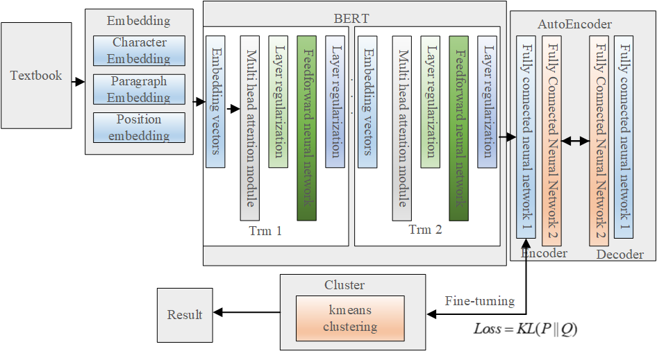
When compared to random initialization, self-coding network initialization of the feature extractor encoder yields superior performance for downstream tasks. The BERT-AE-K-Means model presented in this paper is depicted in Figure 1. It uses the trained EncoderEncoder mentioned above to further reduce the dimensionality of features on the textual data representation, or embedding. It then combines this portion with the Kmeans clustering network to adjust the network parameters inversely based on the clustering results. The following procedure may be used to abstract the process.
Initialize the cluster centers of K-Means clustering algorithm \({\mu _j}\) . Since the division-based K-Means clustering algorithm is very sensitive to the selection of the initial cluster centers, this paper carries out 100 experimental preliminaries using K-Means under different cluster centers, calculates the cluster centers with the smallest division error, and then calculates the probability that point \(i\) belongs to cluster \(j\), \({q_{ij}}\). The calculation formula is shown in Eq. 4 to obtain the probability distribution \(Q\) of the sample points.
\[\label{e4} {q_{ij}} = \frac{{{{\left( {1 + {{\left\| {{z_i} – {\mu _j}} \right\|}^2}/v} \right)}^{ – \frac{{v + 1}}{2}}}}}{{\sum\limits_{{j^\prime }} {{{\left( {1 + {{\left\| {{z_i} – {\mu _{{j^\prime }}}} \right\|}^2}} \right)}^{ – \frac{{v + 1}}{2}}}} }},\tag{4}\] where \({\mu _j}\) stands for the cluster center vector, \({z_i}\) stands for the feature vector of the sample points, and \(v\) is the \(t\) -distribution’s degree of freedom—which, in this work, takes the value of 1.
This paper’s self-supervised learning target distribution uses the auxiliary target distribution \(p\) from the study [15], which is more in line with the original data distribution [], making it a viable choice for an auxiliary target during the self-training phase. Eq. (5) displays the auxiliary target distribution formula:
\[\label{e5} {p_{ij}} = \frac{{q_{ij}^2/\sum\limits_i {{q_{ij}}} }}{{\sum\limits_{{j^\prime }} {\left( {q_{i{j^\prime }}^2/\sum\limits_i {{q_{i{j^\prime }}}} } \right)} }}.\tag{5}\]
The estimated likelihood that sample \(i\) belongs to cluster center \(j\) is indicated by the symbol\({q_{ij}}\) .
Train the clustering network K-Means and the encoder Encoder simultaneously. Since evaluating the disparity between the two distributions is required, this work used the KL-divergence as the loss function to train the model, \(Q\) and \(P\). The KL-divergence is computed as follows in Eq. (6):
\[\label{e6} L = KL(P||Q) = \sum\limits_i {\sum\limits_j {{p_{ij}}} } 1b\frac{{{p_{ij}}}}{{{q_{ij}}}}.\tag{6}\]
If \({q_{ij}}\) is the estimated probability value that sample \(i\) belongs to cluster center \(j\) , \({p_{ij}}\) is the approximate probability that a sample belongs to cluster center \(j\) and \(Q\) is the auxiliary target distribution.
Let \(G = (V,E;\omega ),V = \left\{ {{v_1},{v_2}, \cdots ,{v_n}} \right\}\) be the set of vertices in the network (where \(n\) is an even number of vertices), \({\text{E}} = \left\{ {{e_1},{e_2}, \cdots ,{e_m}} \right\}\) be the set of edges, and \(w = \left\{ {{\omega _1},{\omega _2}, \cdots ,{\omega _m}} \right\}\) be the weight vector of the edges, where \({\omega _i}\) is the weight of the edge \(q\) . A lower constraint on the maximum-right perfect matching is given by \(K\) . The set of perfect matchings is \({M_0}\) (where \(\left| {{M_0}} \right| = \frac{n}{2}\) ). Let \({d_\omega }\left( {{M_0}} \right)\) completely match \({M_0}\) ’s rights in the weight vector \(w\) , that is, \({d_\omega }\left( {{M_0}} \right) = \sum\limits_{{e_k} \in {M_0}} {{\omega _k}}\). To find a new weight vector \(\bar \omega = \left\{ {{{\bar \omega }_1},{{\bar \omega }_2}, \cdots ,{{\bar \omega }_m}} \right\}\) that minimizes the change cost \({\left\| {\bar \omega – w} \right\|_\infty }\) and makes \({M_0}\) a maximum-right perfect match for the network \({G^{\bar \omega }} = (V,E;\bar \omega )\) , this is known as the maximum-right perfect matching inverse problem.
Using the unit \({L_\infty }\) paradigm, the following description of alternating circles is provided before studying the maximum-weight perfect E-matching inverse issue with value constraints:
Definition 1. A circle \(C\) is said to be an alternating circle in a network \(G = (V,E;\omega )\) if it is composed of alternating edges that exactly match \({M_0}\) and edges that are not \({M_0}\) . The weight of the alternating circle \(C\) under the weight vector \(\omega\) is defined as a \({d_\omega }\left[ {\left( {C\backslash {M_0}} \right) – \left( {C \cap {M_0}} \right)} \right]\) , and the edges of circle \(C\) that exactly match \({M_0}\) and the edges that are not \({M_0}\) are denoted as \(C \cap {M_0}\) and \(C\backslash {M_0}\) .
Definition 2. \({d_\omega }\left[ {\left( {C\backslash {M_0}} \right) – \left( {C \cap {M_0}} \right)} \right] = {d_\omega }\left( {C\backslash {M_0}} \right) – {d_\omega }\left( {C \cap {M_0}} \right) \leqslant 0\) indicates that an alternating circle \(C\) is nonpositive if its weight \({d_\omega }\left[ {\left( {C\backslash {M_0}} \right) – \left( {C \cap {M_0}} \right)} \right]\) under the weight vector \(\omega\) is not higher than zero.
For the maximum-weight perfect matching inverse issue, bergel [17] provides the following theorem.
Theorem 1. A prerequisite for \({M_0}\) to be a perfect matching with maximum power in a network \(G = (V,E;\omega )\) is that every alternating circle \(C\) in the network \(G\) must be a nonpositive circle, that is, the alternating circle \(C,{d_\omega }\left[ {\left( {C\backslash {M_0}} \right) – \left( {C \cap {M_0}} \right)} \right] \leqslant 0\).
The following theorem describes how the maximum average alternating circle and the maximum perfect E-matching are related, according to the study [18]:
Proof of Theorem 1. If at any point \({\lambda ^*} \geqslant \mu\), that is, the minimum adjustment of \({\lambda ^*}\) such that the graph \({G^\prime }\) does not have negative circles, has satisfied that the perfect matching \({M_0}\) is a maximum-weighted network matching of the network \({G^{{\omega ^{{\lambda ^*}}}}} = \left( {V,E;{\omega ^{{\lambda ^*}}}} \right)\).
Choose \(p\) as the minimum adjustment cost of the maximum power perfect matching inverse problem with value constraints under the unit \({L_\infty }\) paradigm. This is done when \({\lambda ^*} < \mu\), that is, at this time so that the graph \({G^\prime }\) does not have negative circles of the minimum adjustment amount of the \({\lambda ^*}\), has satisfied the perfect matching \({M_0}\) is the network \({G^{{\omega ^{{\lambda ^*}}}}} = \left( {V,E;{\omega ^{{\lambda ^*}}}} \right)\) of the maximum power network matching, but \({d_{{\omega ^{{\lambda ^*}}}}}\left( {{M_0}} \right) < K\). ◻
As per the previous discussion and Theorem 1, we can obtain the following algorithm for the maximum power perfect matching inverse problem with value constraints under the unit \({L_\infty }\) paradigm by solving \({\mu ^*}\).
In this research, we study four short text datasets through experiments:
Google’s search engine’s SearchSnippets, which has 12,296 brief sentences in all divided into 8 categories.
A collection of title information from a few Q&A situations, available on the Kaggle platform, is called StackOverflow. It has 16,408 brief transcripts from 20 distinct categories in total [].
BioMedical, a dataset from biomedical-related domains that was posted on BioASQ’s official website, with 20 categories and 19,449 samples in total [20].
Tweet is a dataset with 2,474 brief messages divided into 89 categories. Table1 provides comprehensive details on each dataset, with N representing the number of categories, T representing the number of texts, and L representing the average length of the samples in each dataset.
| Dataset | N | T | L |
|---|---|---|---|
| SearchSnippet | 8 | 12296 | 14.42 |
| StackOverflow | 20 | 16408 | 4.05 |
| Tweet | 89 | 2474 | 8.66 |
| Biomedical | 20 | 19449 | 7.41 |
Throughout the experiments presented in this paper, the context-dynamic word vector representations of words are obtained using the BERT pre-training model. Seventy-eight-dimensional vectors derived from the [CLS] labels of the model represent the short text, or text representation containing global information output from the BERT model for text categorization. The current obtained text vector representation is highly dimensional, making direct clustering using the clustering algorithm not only inaccurate but also resulting in a high time complexity of the model. Therefore, this paper suggests using the AutoEncoder model to perform feature extraction and dimensionality reduction of the aforementioned text vectors. The core portion of the self-coding network is split into Encoder and Decoder sections by the AutoEncoder model. The Encoder module has an input layer, hidden layer, and output layer with a total of 768, 1,000, and 128 neurons, respectively.Specifically, the decoder’s input is the encoder’s output. The Decoder module additionally incorporates a three-layer network with 128, 1,000, and 768 neurons, respectively, to accomplish the reconstruction of the vector representation V of the input data. The optimisation strategy applied in the training stage is called stochastic gradient descent (SGD). The feature extractor encoder, which is acquired after thirty optimization rounds, is then utilized to extract features and perform downscaling on the input text vectors V. F
The comparison models are detailed in detail below. This study sets up six groups of comparison experiments, all of which are run on four short text datasets.
The baseline models in the first two comparison groups are Word2Vec and TF-IDF, which provide word vectors, respectively. Based on the word vectors, feature representations of the text are created, and clustering is accomplished directly using the K-Means clustering method.
STC2 is a brief text clustering technique that makes use of word embeddings and convolutional neural networks. Convolutional neural networks are used to learn the text representation throughout the clustering process.
Based on the Dirichlet process, the GSDPMM polynomial mixture model for short text clustering does not need the number of clusters to be predetermined and, as a result of the model’s architecture, typically tends to yield more clusters.
SIF-Auto is a technique that uses SIF word vector format to represent text, then self-coding networks for feature extraction, and clustering as the final step. The paper presents two text representation methods: BERT-K-Means and BERT-AE-K-Means. Both models utilize the pre-trained model BERT to extract the text’s semantic representation; however, the first model differs from the second in that it bypasses the self-coding network for feature extraction and dimensionality reduction. This process verifies the significance of the extracted higher-order features for the downstream text clustering.
The model assessment criteria in this research were clustering accuracy (ACC) and normalized mutual information (NMI), which were determined through many tests on four datasets. The following is the formula for the clustering accuracy ACC:
\[\label{e7} ACC = \frac{{\sum\limits_{i = 1}^N \delta \left( {{y_i},\operatorname{map} \left( {{C_i}} \right)} \right)}}{N},\tag{7}\] where \(N\) is the number of samples, \({y_i}\) is the sample point \({x_i}\)’s actual label, and \({C_i}\) is the cluster label that the model gave to it. Then, \(\operatorname{map} \left( {{C_i}} \right)\) is used to map the cluster label that the model obtained to \({y_i}\) ’s form. Eq. 8 defines the discriminant function \(\delta (x,y)\), which is used to determine if the real label and the category produced from clustering are the same.
\[\label{e8} \delta(x, y)=\left\{\begin{array}{l} 1, \text { if } x=y, \\ 0, \text { otherwise. } \end{array}\right.\tag{8}\]
The following is the typical formula for calculating mutual information NMI:
To normalize the mutual information value to fall within [0,1], \(\sqrt {H(C),H(D)}\) is employed, where \(H( \cdot )\) is the information first.The mutual information value between and is found by calculating\(I(C,D)\).
\[\label{e9} I(C,D) = \sum\limits_{{C_i} \in C,{D_i} \in D} P \left( {{C_i},{D_i}} \right)\operatorname{lb} \frac{{P\left( {{C_i},{D_i}} \right)}}{{P\left( {{C_i}} \right)P\left( {{D_i}} \right)}}.\tag{9}\]
The conventional mutual information value takes the maximum value of 1 when the clustering model separates the data C and D into two pieces properly.
In this paper, six groups of comparison experiments are conducted on the same data set, and the results of the experiments are displayed in Table 2 and Table 3, respectively. The reliability of the experimental results is determined by taking the average of ten experiments as the final results of each model. Three experiments are conducted to confirm the significance of various vector representations of text for text clustering: K-Means, Word2Vec-K-Means, and BERT-K-Means. Table 3 shows that BERT-K-Means performs the best of the three in terms of accuracy, with a 20 percentage point improvement over the Word2Vec-KMeans model and a 24 percentage point improvement over the K-Means model when compared to the SearchSnippet dataset.According to the experimental findings, using word frequency-based text representation directly on short texts yields the lowest results. However, using a large corpus for pre-training can significantly increase the textual representation’s capacity, which in turn increases the effectiveness of text clustering downstream.
| Model | SearchSnippet | StackOverflow | Tweet | Biomedical |
|---|---|---|---|---|
| K-Means | 33.82\(\pm\) 3.90 | 20.29 \(\pm\)3.93 | 41.63 \(\pm\)1.64 | 28.05\(\pm\) 2.79 |
| Word2Vec-K-Means | 53.42 \(\pm\)1.79 | 30.50 \(\pm\)0.31 | 65.72\(\pm\) 2.54 | 33.69 \(\pm\)2.33 |
| GSDPMM | 38.69\(\pm\) 2.75 | 29.35\(\pm\) 1.48 | 84.40\(\pm\) 2.20 | 28.11\(\pm\) 1.79 |
| STC2 | 78.26\(\pm\) 2.69 | 53.82\(\pm\) 3.36 | 75.15 \(\pm\)3.15 | 44.82 \(\pm\)1.73 |
| SIF-Auto | 79.15\(\pm\) 1.25 | 59.88 \(\pm\)1.78 | 77.53 \(\pm\)0.98 | 55.74 \(\pm\)1.96 |
| BERT_K-Means | 78.33\(\pm\) 1.22 | 57.34 \(\pm\)2.12 | 80.32\(\pm\) 2.24 | 52.77\(\pm\) 1.06 |
| BERT_AE_K-Means | 82.29\(\pm\) 1.80 | 63.77\(\pm\) 1.33 | 83.73 \(\pm\)1.64 | 56.66 \(\pm\)0.82 |
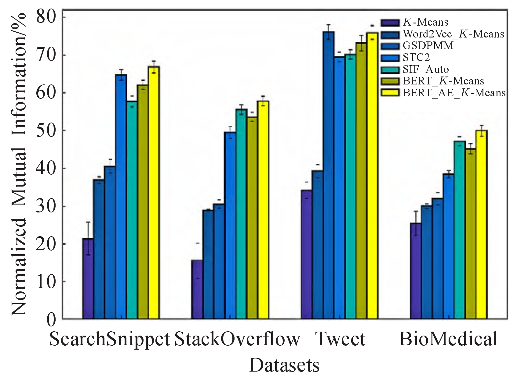
| Model | SearchSnippet | StackOverflow | Tweet | Biomedical |
|---|---|---|---|---|
| K-Means | 21.42\(\pm\) 4.33 | 15.59 \(\pm\)4.67 | 34.25 \(\pm\)2.12 | 25.42 \(\pm\)3.21 |
| Word2Vec-K-Means | 36.92\(\pm\) 0.88 | 28.92\(\pm\) 0.15 | 39.33 \(\pm\)1.83 | 30.11\(\pm\) 0.63 |
| GSDPMM | 40.58\(\pm\) 1.85 | 3.60\(\pm\) 1.15 | 76.14 \(\pm\)1.90 | 32.03 \(\pm\)1.59 |
| STC2 | 64.73\(\pm\) 1.38 | 49.52 \(\pm\)1.64 | 69.45 \(\pm\)1.19 | 38.39\(\pm\) 0.92 |
| SIF-Auto | 57.75 \(\pm\)1.39 | 55.60 \(\pm\)1.22 | 7.14 \(\pm\)1.23 | 47.22 \(\pm\)1.18 |
| BERT_K-Means | 62.12\(\pm\) 1.30 | 53.65\(\pm\) 1.14 | 73.22\(\pm\) 2.08 | 45.17 \(\pm\)1.53 |
| BERT_AE_K-Means | 66.86\(\pm\) 1.51 | 57.82\(\pm\) 1.22 | 75.96\(\pm\) 1.69 | 50.02 \(\pm\)1.46 |
The methods that have been proposed in recent years to achieve good results on these four datasets are known as experiments GSDPMM, STC2, and SIF-Auto. These methods are used in Table 2and Table 3 to validate the effectiveness of the feature extraction and clustering methods proposed in this paper. It is evident that GSDPMM performs best on the Tweet dataset because it contains 89 categories, which is four times more samples than the other datasets. The GSDPMM model also tends to produce more clusters, which helps it achieve the best results on this data, where both the ACC and NMI values are less than 1 percentage point higher than the model that is proposed in this paper. The approach suggested in this paper produces the best results on the remaining three datasets: on the StackOverFlow dataset, the ACC improves by 3 percentage points over the results of the best comparison model, SIF-Auto, and on the BioMedical dataset, the NMI value improves by 2.8 percentage points over the results of the comparison model, SIF_Auto.
The efficacy of the self-coding network suggested in this paper for text feature extraction and dimensionality reduction is finally verified by comparing two sets of experiments, BERT_K-Means and BERT_AE_KMeans. The representation vector of the text is better suited for downstream applications following feature extraction and dimensionality reduction through this module. The clustering accuracy is improved on all datasets, as Tables 2 and 3 demonstrate. The three datasets with the exception of the Tweet dataset yielded the best comparison experiment results, with the NMI value on the StackOverflow dataset increasing by more than 4 percentage points when compared to BERT_K-Means and the ACC increasing by 6 percentage points. It demonstrates how the dimensionality reduction and feature extraction approach for text representation put forward in this work may successfully enhance text representation capabilities, enhancing the clustering algorithm’s performance.
The aforementioned experiments confirm the usefulness of the text representation and higher-order feature extraction techniques suggested in this paper in terms of enhancing clustering accuracy. In addition, this paper chooses the comparative experiments STC2 and SIF_Auto, which were proposed recently, as well as the BERT_K-Means and BERT_AE_K-Means models, which are proposed here, to conduct runtime tests on each of the four datasets with 10,000 samples. The comparison results are displayed in Figure 2.
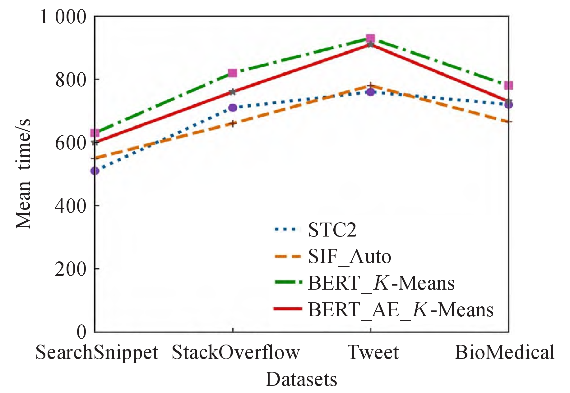
Figure 2 illustrates that the BERT_AE_KMeans model proposed in this paper has a lower running time than BERT_K-Means on the four datasets, and a slightly longer running time than the two comparison experiments of STC2 and SIF_Auto. This is because the BERT pre-training model produces 768-dimensional high-dimensional feature vectors, which need more computation time. In contrast to BERT_K-Means, in this paper, after extracting the higher-order features by AutoEncoder module, not only does the computation amount decrease, but also the clustering model is easier to converge, resulting in a lower running time than the BERT_K-Means model. Therefore, it can be seen that the model proposed in this paper does not substantially increase the time complexity while improving the clustering accuracy.
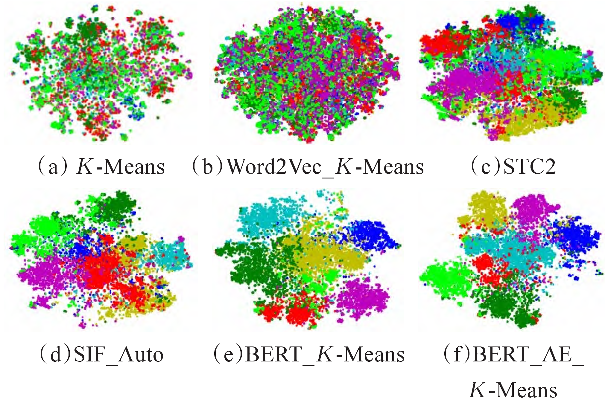
For the dimensionality reduction process, the features of the sample data are reduced to a 2-dimensional space by using the integrated model t-SNE in the Python Sklearn library. This allows for a more intuitive understanding of the changes in the clustering results. This paper conducts a comparative experiment on the clustering results under the SearchSnippet dataset. The visualization effect is displayed in Figure 3. The STC2 model uses convolutional networks to extract the features of the textual information, as compared with (a). For the short text dataset, the sample data contains fewer words, and the core words that can reflect the meaning of the text are insufficient. The text vectorization feature method through word frequency statistics results in a low weight reflecting the core semantic words. In contrast to (b), the clustering method operates directly on the data space, resulting in a more pronounced clustering impact and distinct border curves for each cluster once the former characteristics are extracted. After extracting the text’s higher-order feature representation using the self-coding network, (d) employs SIF for text representation, therefore enhancing the clustering impact. When compared to (b), it is evident that the pre-trained model BERT uses contextual environment information to dynamically obtain the text representation that is more conducive to downstream clustering than that obtained by using Word2Vec, and that the boundaries of the individual clusters are more clearly defined. (e) illustrates this process of using K-Means for clustering after adopting the pre-trained model BERT for text representation in this paper. The clustering results produced by the BERT_AE_K-Means model, which is suggested in this study, are shown in (f). By comparing with (e), it is further confirmed that the clustering model’s effectiveness can be further enhanced by extracting the higher-order features for the text vectors obtained by BERT using the self-coding network. The clustering results demonstrate the best effect in the SearchSnippet dataset, and the obtained cluster boundaries are more distinct. The resultant clusters’ borders are more distinct.
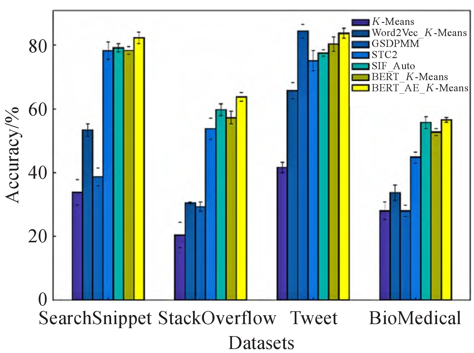
The aforementioned experiments indicate that the vectorized characterization of text is crucial for the text clustering task. This paper fully utilizes the large pre-training model BERT to extract the high dimensional space between words of the semantic and syntactic and other information, which is especially important for the downstream text clustering task to improve the clustering task’s effect. The accuracy on the text clustering problem has significantly increased, along with the feature extraction, dimensionality reduction, and clustering fine-tuning approaches suggested in this study. As seen in Figures 4 and 5, which depict the longitudinal comparison results of clustering accuracy and standard mutual information value in each model, we can infer from these that the model that is suggested in this study achieves a greater accuracy rate.
In this work, we examine how deep learning and self-supervised learning are used to text clustering and conclude that both techniques are critical to enhancing text representation and clustering outcomes. A more accurate and enhanced representation is supplied for the text clustering job to better capture the syntactic and semantic information of the text. Deep learning models are able to better interpret the semantic and contextual information of text, which enhances the text clustering impact when compared to the standard approaches based on word frequency statistics. The approach in this study may better use the internal structure and features of the data by doing text clustering trials, which will increase the accuracy and efficiency of clustering.
The experimental data used to support the findings of this study are available from the corresponding author upon request.