
In this paper we are only concerned with simple undirected graphs with finite number of vertices. We follow [1] for all notation not described here. As usual, the complete graph on \(n\) vertices is denoted \(K_n\), and the complete bipartite graph whose partite sets have order \(s\) and \(t\) is denoted \(K_{s,t}\). We use the notation \(K_{2,t}+uv\) to mean the graph obtained from \(K_{2,t}\) by adding an edge between the vertices in the partite set of order \(2\). For two graphs \(G\) and \(H\), the union of \(G\) and \(H\), denoted \(G\cup H\), is the graph with \(V(G\cup H)=V(G)\cup V(H)\) and \(E(G\cup H)=E(G)\cup E(H)\). For some \(k\ge 2\), the union of \(k\) copies of a graph \(G\) is denoted \(kG\). The join of two graphs \(G\) and \(H\), written \(G\vee H\), is the graph obtained from \(G\cup H\) by adding all edges between vertices of \(G\) and vertices of \(H\).
We are mostly concerned with colorings of the edges of a graph using two colors. We follow the convention that the two colors used are red and blue and refer to such colorings as red-blue colorings of \(G\). Given a red-blue coloring \(\mathcal{C}\) of \(G\), the graphs induced by the red and blue edges are denoted \(G_r\) and \(G_b\), respectively.
A graph \(G\) is said to arrow the graphs \(F\) and \(H\), denoted \(G\rightarrow (F,H)\) if every red-blue coloring of \(G\) has the property that either \(F\) is isomorphic to a subgraph of \(G_r\) or \(H\) is isomorphic to a subgraph of \(G_b\). The Ramsey number of \(F\) and \(H\), denoted \(R(F,H)\), is the smallest positive integer \(n\) for which \(K_n\rightarrow (F,H)\). The existence of such a number is guaranteed by the classical result of Frank Ramsey [2]. The Ramsey number just described is referred to as a Classical Ramsey Number and has been extensively studied. As well, a number of variations of the topic have been introduced (see [3] for a dynamic survey of Ramsey theory by Radzisowski).
Of particular interest in Ramsey theory are the diagonal Ramsey numbers, that is, Ramsey numbers of the form \(R(F,F)\) for a graph \(F\). It is well known that \(R(K_3,K_3)=6\), and Greenwood and Gleason proved \(R(K_4,K_4)=18\) in 1955 [4]. The Ramsey number \(R(K_5,K_5)\) is, at the date of this writing, still unknown. However, it is known that \(43\le R(K_5,K_5)\le 48\) (see [5] and [6] for the lower and upper bounds respectively). While we offer no new bounds on this Ramsey number, we introduce a concept in order to approach diagonal Ramsey numbers from a new perspective.
Here, rather than find the smallest integer \(n\) for which \(K_n\rightarrow (H,H)\), we instead fix a graph \(G\) and find all graphs \(H\) for which \(G\rightarrow (H,H)\), or simply \(G\rightarrow H\). For example, it is known that \(R(C_4,C_4)=6\) [7]. It follows that every red-blue coloring of \(K_7\) contains a monochromatic \(C_4\). As well, \(R(K_3,K_3)=6\). So, every red-blue coloring of \(K_7\) contains a monochromatic \(K_3\). Of course, all subgraphs of \(K_3\) and \(C_4\) must also appear in either the red or blue subgraph in any coloring of \(K_7\). We ask the question: Is this a complete list? What graphs, that do not fit into common families of graphs covered by the Radzisowski survey, are missing when we consider every red-blue coloring of \(K_7\)? We approach this problem through the lens of order theory by first considering the partially ordered set (poset) of graphs which are subgraphs of some graph \(G\). This generalizes the work of Steinbach [8] who determined the poset of graphs for \(K_n\) when \(n\le 8\). See also [9] for this poset when \(n=9\).
We determine the down-arrow Ramsey set for several classes of graphs \(G\), in particular, when \(G\) is a cycle or a path of any order and when \(G\) is a complete graph of order \(n\le 7\). As a consequence of our results for complete graphs, we have determined all graphs with Ramsey number at most \(n\) for all \(n\le 7\).
For a fixed graph \(G\), we define the down-arrow Ramsey set of \(G\), denoted \(\downarrow G\), as the set of graphs \(H\) for which \(G\rightarrow H\). that is, \[\downarrow G=\{H\subseteq G\ :\ G\rightarrow H\}.\]
From this definition, the connection to traditional Ramsey theory is immediate.
Observation 1. Let \(G\) be a graph without isolated vertices. Then, \(R(G,G)=n\) if and only if \(n\) is the smallest positive integer for which \(G\in \ \downarrow K_n\).
Additionally, some properties of inclusion follow from the definition of the down-arrow Ramsey set.
Observation 2. If \(H\subseteq G\), then \(\downarrow H\subseteq\ \downarrow G\).
Observation 3. If \(H\in \ \downarrow G\), then \(F\in\ \downarrow G\) for all \(F\subseteq H\).
Observation 3 offers a method for describing the down-arrow Ramsey set. that is, we identify the maximal elements of \(\downarrow G\) so that all elements of the set are guaranteed to be subgraphs of one of the maximal elements. Hence, we borrow language from order theory in order to formalize this idea. Given a graph \(G\), let \(\langle G\rangle\) be the set of all isomorphism classes of graphs which are subgraphs of \(G\). This set forms a partially ordered set under the relation “is isomorphic to a subgraph of”, which we denote “\(\subseteq\)“. Now, if \(G\) is a graph of order \(n\), then \(G\subseteq K_n\), and hence \(\langle G\rangle \subseteq \langle K_n\rangle\). Noting Observation 3, we see that \(\langle G\rangle\) is downwardly closed. Further, any two graphs \(F\) and \(H\) in \(\langle G\rangle\) have a common supergraph in \(\langle G\rangle\), namely \(G\). This establishes the following observation.
Observation 4. The partially ordered set \(\langle G\rangle\) is an order ideal of the partially ordered set \(\langle K_n\rangle\).
Being the smallest poset that contains \(G\), \(\langle G\rangle\) is called the principle ideal generated \(G\), which we refer to as a graph ideal. So, we can describe \(\downarrow G\) as a union of graph ideals. However, the use of order theory here is not superficial. Our main method for determining the down-arrow Ramsey set relies on viewing red-blue colorings of a graph as unions of graph ideals.
Observation 5. If \(\mathcal{C}\) is a red-blue coloring of a graph \(G\), with red subgraph \(G_R\) and blue subgraph \(G_B\), then \(\downarrow G\subseteq \langle G_R\rangle \cup \langle G_B \rangle\).
In determining \(\downarrow G\), it is necessary to consider multiple red-blue colorings of a graph \(G\). The following observation comes from applying Observation 5 to more than one red-blue coloring of \(G\). Notice here that we can think of a coloring \(\mathcal{C}\) as the union of ideals generated by its red and blue subgraphs, i.e. \(\mathcal{C}=\langle G_r\rangle \cup \langle G_b\rangle .\)
Observation 6. Suppose \(\mathcal{C}_1,\mathcal{C}_2,\ldots \mathcal{C}_k\) are \(k\) red-blue colorings of the graph \(G\), in which each \(\mathcal{C}_i\) decomposes \(G\) into \(G_{R_i}\) and \(G_{B_i}\). Then \[\downarrow G\subseteq \bigcap_{i=1}^k \mathcal{C}_i=\bigcap_{i=1}^k\left(\langle G_{r_i}\rangle\cup \langle G_{b_i}\rangle \right)\]
In fact, even more can be said. If we take as our collection of colorings the set of all red-blue colorings of \(G\), then this intersection is exactly \(\downarrow G\). Indeed, if a graph \(H\) is not in \(\downarrow G\), then there must be some coloring \(\mathcal{C}\) for which \(H\notin \langle G_r\rangle\) and \(H\notin \langle G_b\rangle\). This establishes the following proposition.
Proposition 1. Given a nonempty graph \(G\) on \(n\ge 2\) vertices, there exists a finite set set of colorings \(\{\mathcal{C}_i\}_{i=1}^k\) of \(G\) for which \[\downarrow G=\bigcap_{i=1}^k \mathcal{C}_i=\bigcap_{i=1}^k\left(\langle G_{r_i}\rangle\cup \langle G_{b_i}\rangle \right).\]
Proposition 1 reveals that we need only develop an efficient method for reducing intersections of graph ideals as unions of graph ideals. However, the set of all red-blue colorings can be quite large, even for small order graphs, and so it would be computationally difficult to consider all of them. Instead, for a given graph \(G\) we seek to determine a small number of colorings of \(G\) for which an application of Proposition 1 reveals exactly \(\downarrow G\). However, this implies that we must first find the maximal elements of \(\downarrow G\) through traditional means. The main use for Proposition 1 is then to show that we have actually identified the maximal elements, that is, that there are no other elements in \(\downarrow G\).
With these considerations, it was necessary to develop a rigorous method for determining graph ideal intersections by hand. Some ideal intersections are obvious, while others require more work. Most intersections used in this paper can be approached by drawing Hasse diagrams, an example of which is shown below. In more general situations, such as \(\downarrow C_n\), explanations are given for the non-trivial intersections used and are presented as lemmas. The following observation is useful for simplifying graph ideal intersections.
Proposition 2. Let \(G\) and \(H\) be graphs with \(H\subseteq G\). Then \(\langle H\rangle \cap \langle G\rangle =\langle H\rangle\)
Next, we see an example of how Hasse diagrams may be used to compute intersections of specific graphs. This is a convenient point to mention that in the determination of graph ideal intersections we do not write the isolated vertices in any ideal intersection. Since all red-blue colorings are of a particular graph, in the next example \(K_6\), it may be assumed that all graphs have the same number of vertices as the host graph.
Example 1. We determine the graph ideal intersections below.
\(\langle K_{2,4}+uv\rangle \cap \langle K_5\rangle =\langle K_{2,3}+uv\rangle\)
\(\langle K_{3,3}\rangle \cap \langle K_{2,3}+uv\rangle =\langle K_{2,3}\rangle\)
\(\langle K_{3,3}\rangle \cap \langle K_4\rangle =\langle K_{1,3}\rangle \cup \langle K_{2,2}\rangle\)
\(\langle K_3\cup K_3\rangle \cap \langle K_{2,3}+uv\rangle =\langle K_3\rangle \cup \langle 2K_2\rangle\)
\(\langle K_{3}\cup K_3\rangle \cap \langle K_4\rangle = \langle K_3\rangle \cup \langle 2K_2\rangle\)
\(\langle K_{2,3}\rangle \cap \langle f_5\rangle =\langle K_{2,3}-e\rangle\)
Here, \(f_5\) is the fan graph on 6 vertices obtained by joining a vertex to a \(P_5\). Equivalently, \(f_5\cong P_5\vee K_1\).
In each of the following diagrams, let double arrows represent vertex-deleted subgraphs, single arrows represent edge-deleted subgraphs, and dashed lines indicate a graph in the Hasse diagram where a subgraph of the arrow’s tail appears.
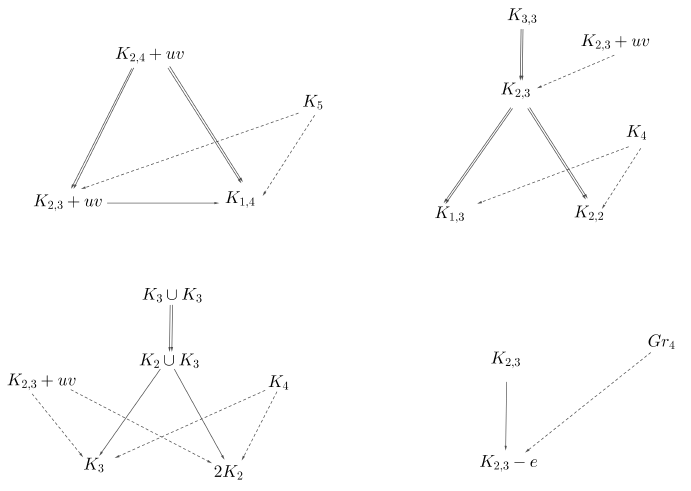
As depicted in the diagram (a), we can determine intersection (1) by first writing \(K_{2,4}+uv\). Since \(K_5\) has only \(5\) vertices while \(K_{2,4}+uv\) has 6, we are able to consider vertex-deleted subgraphs of \(K_{2,4}+uv\) and be sure that no intermediate graphs will be subgraphs of \(K_5\). Up to isomorphism, there are only two options for these vertex-deleted subgraphs. Both resulting subgraphs are subgraphs of \(K_5\). Since \(K_{1,4}\) is also a subgraph of \(K_{2,3}+uv\), it is clear that this intersection is generated by \(K_{2,3}+uv\). In diagrams (b) and (c) and (d), we follow a similar process. Diagrams (b) and (c) show that we can determine multiple intersections with the same diagram. Care must be taken in diagram (c) since we use both vertex- and edge-deleted subgraphs. Generally, we consider vertex-deleted subgraphs until the order of the subgraphs match the order of the graph with which we are intersecting. We then consider edge-deleted subgraphs.
In this section, we determine the down-arrow Ramsey sets of cycles and paths. First we consider cycles of even order.
Theorem 7. The down-arrow Ramsey set \(\downarrow C_n =\langle \lceil \frac{n}{4}\rceil K_2\rangle\) for all even \(n\geq 4\).
Proof. First, consider the red-blue coloring of \(C_n\) for which the red and blue subgraphs are both \(P_{\frac{n}{2}+1}\). Thus, if \(G \in \ \downarrow C_n\), then \(G\subseteq P_{\frac{n}{2}+1}\). Additionally, consider the red-blue coloring of the edges of \(C_n\) such that both the red and blue subgraphs are \(\frac{n}{2}\) disjoint copies of \(K_2\). This implies that if \(G \in \downarrow C_n\), then \(G\subseteq (\frac{n}{2}) K_2\). Therefore, if \(G \in \downarrow C_n\), then these two requirements imply that in fact \(G\subseteq \lceil\frac{n}{4}\rceil K_2\).
Now, we show that \(\lceil\frac{n}{4}\rceil K_2 \in \ \downarrow C_n\). Let there be any red-blue coloring of \(C_n\). Then, there must be at least \(\frac{n}{2}\) edges of the same color. Say there are \(k\geq \frac{n}{2}\) blue edges. Then at least \(\lceil \frac{k}{2}\rceil\) of these edges are independent, which implies that there are at least \(\lceil \frac{k}{2}\rceil \geq \lceil \frac{n}{4}\rceil\) independent blue edges. Therefore, we have a monochromatic \(\lceil \frac{n}{4}\rceil K_2\). ◻
Next, we determine \(\downarrow C_n\) for odd \(n\), which proves more difficult than even \(n\). We consider the case when \(n=3\) separately.
Proposition 3. The down-arrow Ramsey set \(\downarrow C_3=\langle P_3\rangle\).
Proof. Suppose there is a red-blue coloring of \(C_3\) whose color classes are \(G_r\) and \(G_b\). Since \(C_3\) has 3 edges, it follows that some color class has at least two edges. Without loss of generality, assume that \(G_r\) has two edges. Then we have two adjacent red edges, hence a red \(P_3\). This shows \(\langle P_3\rangle \subseteq \ \downarrow C_3\). For the reverse inclusion, let \(G \in \ \downarrow K_3\). The red-blue coloring of \(C_3\) with \(P_3\) as the red subgraph and \(K_2\) as the blue subgraph shows that either \(G\subseteq P_3\) or \(G\subseteq K_2\). Hence, \(G\subseteq \langle P_3\rangle\). ◻
Now, we show that \(P_3 \cup \lfloor \frac{n-3}{4} \rfloor K_2\) and \(\lceil \frac{n}{4} \rceil K_2\) are in the down-arrow Ramsey set of all odd cycles of order \(n\geq 5\).
Lemma 1. For all odd \(n\geq 5\), \(\langle P_3 \cup \lfloor \frac{n-3}{4} \rfloor K_2 \rangle \cup \langle \lceil \frac{n}{4} \rceil K_2 \rangle \subseteq \ \downarrow C_n\).
Proof. It follows from a similar argument from above that \(\langle\lceil \frac{n}{4} \rceil K_2 \rangle \in \ \downarrow C_n\) for odd \(n\) as well.
To show that \(P_3 \cup \lfloor \frac{n-3}{4} \rfloor K_2\) must be in \(\downarrow C_n\), we consider two cases, depending on the order of \(C_n\) modulo 4.
Case 1: Suppose \(n=4k+1\), for \(k\geq 1\). Note that \(\lfloor \frac{n-3}{4} \rfloor=k-1\) in this case, so we are aiming to show that \(P_3 \cup (k-1) K_2 \in \ \downarrow C_n\). Let there be a red-blue coloring of \(C_n\). We know that there are at least \(\lceil \frac{n}{2} \rceil=2k+1\) edges of one color. Without loss of generality, say there are at least \(2k+1\) blue edges. Of these blue edges, at least \(k+1\) of them are independent. Let \(S=\{ e_1, e_2, \ldots e_k, e_{k+1}\}\) be a set of \(k+1\) independent blue edges.
Since the independence number of \(C_n\) is \(\lfloor \frac{n}{2}\rfloor=2k\), then we know there are at most \(2k\) independent blue edges. Hence, there are at least two blue edges that are adjacent to each other. Label these edges as \(a\) and \(b\), and label the other edges adjacent to \(a\) and \(b\) to be \(c\) and \(d\) respectively. Notice that at most two of the four edges \(a\), \(b\), \(c\), \(d\) are in the set \(S\) of independent blue edges. Thus, if \(k>1\), then there are still at least \(k-1\) independent blue edges that are not \(a\), \(b\), \(c\), or \(d\). Therefore these independent edges together with \(a\) and \(b\) form a blue \(P_3 \cup (k-1) K_2\). If \(k=1\), then we have formed a blue \(P_3\) with edges \(a\) and \(b\), which follows the statement of the lemma.
Case 2: Suppose \(n=4k+3\), for \(k\geq 1\). Here we have \(\lfloor \frac{n-3}{4} \rfloor=k\) in this case, so we need to show that \(P_3 \cup k K_2 \in \ \downarrow C_n\). Let there be a red-blue coloring of \(C_n\). We must have at least \(\lceil \frac{n}{2} \rceil = 2k+2\) edges of one color, say blue. Of these blue edges, we have that at least \(k+1\) of them are independent and at most \(\lfloor \frac{n}{2} \rfloor=2k+1\) of them are independent.
Notice that if there are at least \(k+2\) independent blue edges, then we could use the same argument in the previous case to show that there must be a blue \(P_3 \cup k K_2\). Assume that there are exactly \(k+1\) independent blue edges, and let \(S=\{e_1, e_2, \ldots , e_k, e_{k+1}\}\) be the set of all independent blue edges. Since there are at least \(2k+2\) blue edges, this means that there are at least \(k+1\) blue edges that are adjacent to one or more blue edges in \(S\). It follows that there must be at least one blue edge that is adjacent to exactly one edge in \(S\). Call this edge \(f\), and suppose it is adjacent to \(e_j\), \(1\leq j \leq k+1\). Thus, the set of edges \(S-e_j\) forms a blue \(k K_2\) and \(f\) and \(e_j\) together form a blue \(P_3\). Therefore, we have a blue \(P_3 \cup k K_2\). ◻
Using three red-blue colorings of an odd cycle and intersections of the ideals generated by their red and blue subgraphs, we show that any graph in the down-arrow Ramsey set of an odd cycle \(C_n\) must be a subgraph of \(P_3 \cup \lfloor \frac{n-3}{4} \rfloor K_2\) or \(\lceil \frac{n}{4} \rceil K_2\) to finish the following theorem. In order to justify the graph ideal intersection used in the proof of the theorem, we present the following two lemmas.
Lemma 2. Let \(n\ge 5\) be an odd positive integer, then
\(\langle \left(\frac{n-3}{2}\right) K_2\cup P_3\rangle \cap \langle P_{\frac{n-1}{2}}\cup P_3\rangle= \langle \lfloor \frac{n-1}{4}\rfloor K_2\cup P_3 \rangle.\)
Proof. Let \(G_1=\left(\frac{n-3}{2}\right) K_2\cup P_3\) and \(G_2=P_{\frac{n-1}{2}}\cup P_3\). It is clear that the reverse inclusion holds. For the forward inclusion, let \(H\in \langle G_1\rangle \cap \langle G_2\rangle\) and notice that the edge independence number of \(G_2\) is \(\lfloor \frac{n-1}{4}\rfloor +1=\lfloor \frac{n+3}{4}\rfloor\). Hence, the edge independence number of \(H\) is at most \(\lfloor \frac{n+3}{4}\rfloor\). Since \(H\) is also a subgraph of \(G_1\) it follows that \(H\) is a subgraph of \(\lfloor \frac{n+3}{4}\rfloor K_2\) or a subgraph of \(\lfloor \frac{n-1}{4}\rfloor K_2\cup P_3\). Since \(\lfloor \frac{n+3}{4}\rfloor K_2\) is a subgraph of the latter graph, the result holds. ◻
Lemma 3. Let \(n\ge 5\) be an odd positive integer, then
\(\langle P_{\frac{n+3}{2}}\rangle \cap \langle \lfloor \frac{n-1}{4}\rfloor K_2\cup P_3\rangle = \langle \lfloor \frac{n+3}{4}\rfloor K_2\rangle \cup \langle \lfloor \frac{n-3}{4} \rfloor K_2\cup P_3\rangle\).
Proof. Let \(G_1=P_{\frac{n+3}{2}}\) and \(G_2=\lfloor \frac{n-1}{4}\rfloor K_2\cup P_3\). It is clear that the reverse inclusion holds. For the forward inclusion, we consider two cases depending on whether \(n\equiv 1\pmod 4\) or \(n\equiv 3\pmod 4\).
Case 1: Suppose \(n=4k+1\), for \(k\geq 1\). In this case \(G_1=P_{2k+2}\) and \(G_2=k K_2\cup P_3\). Notice that deleting any edge of \(G_2\) yields either \((k+1) K_2\) or \((k-1)K_2\cup P_3\) and that each of these is a subgraph of \(P_{2k+2}\), while \(G_2\) itself is not. Finally, notice that \(k-1=\frac{n-5}{4}=\lfloor \frac{n-3}{4}\rfloor\) and \(k+1=\lfloor \frac{n+3}{4}\rfloor\) when \(n=4k+1\).
Case 2: Suppose \(n=4k+3\), for \(k\geq 1\). In this case \(G_1=P_{2k+3}\) and \(G_2=k K_2\cup P_3\). Hence, \(G_2\subseteq G_1\) and so \(\langle G_2\rangle \cap \langle G_1\rangle =\langle G_2\rangle\). However, \(\lfloor \frac{n+3}{4}\rfloor K_2 = (k+1)K_2\) and \(\lfloor \frac{n-3}{4}\rfloor K_2\cup P_3 = k K_2\cup P_3\). Since \((k+1)K_2\subseteq k K_2\cup P_3=G_2\), the result holds here as well. ◻
Theorem 8. The down-arrow Ramsey set \(\downarrow C_n=\langle P_3 \cup \lfloor \frac{n-3}{4} \rfloor K_2 \rangle \cup \langle \lceil \frac{n}{4} \rceil K_2 \rangle\) for all odd \(n\geq 5\).
Proof. Due to Lemma 1, it suffices to show that \(\downarrow C_n \subseteq \langle P_3 \cup \lfloor \frac{n-3}{4} \rfloor K_2 \rangle \cup \langle \lceil \frac{n}{4} \rceil K_2 \rangle\).
Consider the following three red-blue colorings of \(C_n\):
\(\mathcal{C}_1\): \(G_{r_1}\cong P_{\frac{n+1}{2}}\),\(G_{b_1}\cong P_{\frac{n+3}{2}}\)
\(\mathcal{C}_2\): \(G_{r_2}\cong\left(\frac{n-1}{2}\right)K_2\),\(G_{b_2}\cong\left(\frac{n-3}{2}\right)K_2\cup P_3\)
\(\mathcal{C}_3\): \(G_{r_3}\cong P_{\frac{n-3}{2}}\cup P_3\),\(G_{b_3}\cong P_{\frac{n-1}{2}}\cup P_3\)
Notice first that \(G_{r_1}\subseteq G_{b_1}\), \(G_{r_2}\subseteq G_{b_2}\), and \(G_{r_3}\subseteq G_{b_3}.\) Hence, for odd \(n\), \[\begin{aligned} \downarrow C_n\subseteq \mathcal{C}_1\cap \mathcal{C}_2\cap \mathcal{C}_3&=\left\langle G_{b_1}\right\rangle \cap \langle G_{b_2}\rangle \cap \langle G_{b_3}\rangle \\ &=\left\langle P_{\frac{n+3}{2}}\right\rangle \cap \left(\left\langle \left(\frac{n-3}{2}\right)K_2\cup P_3\right\rangle \cap \left\langle P_{\frac{n-1}{2}}\cup P_3 \right\rangle \right)\\ &=\left\langle P_{\frac{n+3}{2}}\right\rangle\cap \left\langle \left\lfloor \dfrac{n-1}{4}\right\rfloor K_2 \cup P_3\right\rangle\\ &=\left\langle \left\lfloor\dfrac{n+3}{4}\right\rfloor K_2\right\rangle\cup \left\langle \left\lfloor \dfrac{n-3}{4}\right\rfloor K_2 \cup P_3 \right\rangle \end{aligned}\]
Finally, notice that when \(n\) is odd, \(\left\lfloor \frac{n+3}{4} \right\rfloor=\left\lceil \frac{n}{4}\right\rceil\). ◻
By using a similar argument as was used for cycles, we can see that there must be a monochromatic \(\lceil \frac{n-1}{4}\rceil K_2\) in every red-blue coloring of \(P_n\). This tells us that \(\langle \lceil \frac{n-1}{4}\rceil K_2 \rangle \subseteq \ \downarrow P_n\). In fact, we can also show that anything in the down-arrow Ramsey set of \(P_n\) must be in \(\langle \lceil \frac{n-1}{4}\rceil K_2 \rangle\), giving us the following result.
Proposition 4. The down-arrow Ramsey set \(\downarrow P_n =\langle \lceil \frac{n-1}{4}\rceil K_2 \rangle\) for all \(n\geq 3\).
Proof. We can see that \(\langle \lceil \frac{n-1}{4}\rceil K_2 \rangle \subseteq \ \downarrow P_n\). Now, let \(G\) be a graph in the down-arrow Ramsey set of \(P_n\). We will use two red-blue colorings of \(P_n\) to show \(G \subseteq \lceil \frac{n-1}{4}\rceil K_2\).
For ease of notation, let \(k=\lfloor\frac{n-1}{2}\rfloor\) and \(k'=\lceil\frac{n-1}{2}\rceil\). Consider the red-blue coloring of the edges of \(P_n\) for which the red subgraph is \(P_{k'+1}\) and the blue subgraph is \(P_{k+1}\). This implies that \(G \subseteq P_{k+1}\). Additionally, consider the red-blue coloring of the edges of \(P_n\) for which the red subgraph is \((k')K_2\) and the blue subgraph is \(k K_2\). This coloring suggests that we also have \(G \subseteq k K_2\). Hence,
\(G \subseteq \langle P_{k+1} \rangle \cap \langle k K_2 \rangle = \langle \lceil \frac{k}{2}\rceil K_2 \rangle=\langle \lceil \frac{n-1}{4}\rceil K_2 \rangle\).
Therefore we have \(\downarrow P_n =\langle \lceil \frac{n-1}{4}\rceil K_2 \rangle\). ◻
In this section, we investigate the down-arrow Ramsey sets of complete graphs up to order 8. This section has the most connection to traditional Ramsey theory. Recall that in calculating the down-arrow Ramsey set of \(K_n\), we are able to describe all graphs \(G\) for which \(R(G,G)\le n\) for \(n\le 8\).
Since there are no nonempty proper subgraphs of \(K_2\), we observe the following:
Observation 9. The down-arrow Ramsey set \(\downarrow K_2=\langle\overline{K_2}\rangle\).
Since \(C_3=K_3\), we already know that the down-arrow Ramsey set \(\downarrow K_3=\langle P_3\rangle\) from Lemma 3. Next, we consider the complete graph on four vertices.
Proposition 5. The down-arrow Ramsey set \(\downarrow K_4=\langle P_3\rangle\).
Proof. By Proposition 3 it follows that \(\langle P_3 \rangle \subseteq \ \downarrow K_4\). To see the reverse inclusion, consider the following two red-blue colorings of the edges of \(K_4\).
\(G_{r_1}\cong G_{b_1}\cong P_4\)
\(G_{r_2}\cong K_3\), \(G_{b_2}\cong K_{1,3}\)
So, \[\begin{aligned} \downarrow {K_4}&\subseteq \left(\langle K_3\rangle \cup \langle K_{1,3}\rangle\right)\cap \langle P_4\rangle\\ &=\left(\langle K_3\rangle \cap \langle P_4\rangle \right)\cup \left(\langle K_{1,3}\rangle \cap \langle \langle P_4\rangle \right)\\ &=\langle P_3\rangle \cup \langle P_3\rangle\\ &=\langle P_3\rangle \end{aligned}\] Thus, \(\downarrow K_4=\langle P_3\rangle\), as desired. ◻
Proposition 6. The down-arrow Ramsey set \(\downarrow K_5=\langle P_4\rangle\).
Proof. We first show that \(P_4\in \ \downarrow K_5\). Assume to the contrary that there is a red-blue coloring of \(K_5\) that avoids a monochromatic \(P_4\). Label the vertices of \(K_5\) by \(v_1,v_2,v_3,v_4,\) and \(v_5\). By Proposition 5, we are guaranteed a monochromatic \(P_3\). So, we may assume that \(v_1v_2\) and \(v_2v_3\) are red edges. If any of the edges \(v_1v_4\),\(v_1v_5\), \(v_3v_5\), or \(v_4v_5\) are red, then we have a red \(P_4\). Hence, each of these edges is blue. However, then \((v_4, v_1, v_5, v_3)\) is a blue \(P_4\). So, we have that \(P_4\in \ \downarrow K_5\) and hence \(\langle P_4\rangle \subseteq \ \downarrow K_5\).
To see the reverse inclusion, consider the following red-blue colorings of the edges of \(K_5\):
\(G_{r_1}\cong G_{b_1}\cong C_5\)
\(G_{r_2}\cong K_4\), \(G_{b_2}\cong K_{1,4}\)
So, \[\begin{aligned} \downarrow K_5\subseteq \langle C_5\rangle\cap \left(\langle K_4\rangle\cup\langle K_{1,4}\rangle \right)&=\left(\langle C_5\rangle \cap \langle K_4\rangle\right)\cup \left(\langle C_5\rangle \cap \langle K_{1,4}\rangle\right)\\ &=\langle P_4\rangle \cup \langle P_3\rangle\\ &=\langle P_4\rangle \end{aligned}\] Thus, \(\downarrow K_5=\langle P_4\rangle\), as desired. ◻
The determination of the down-arrow Ramsey sets for \(K_n\) thus far have been fairly straight-forward. However, the determination of the next two down-arrow Ramsey sets, \(\downarrow K_6\) and \(\downarrow K_7\), are more involved.
Lemma 4. \(K_{2,3}-e \in \ \downarrow K_6\) and \(K_3 \in \ \downarrow K_6\). In other words, \(\langle K_{2,3}-e \rangle \cup \langle K_3\rangle \subseteq \ \downarrow K_6\).
Proof. Clearly, \(K_3 \in \ \downarrow K_6\) since the Ramsey number \(R(K_3, K_3)=6\). To see that \(K_{2,3}-e \in \ \downarrow K_6\), first note that \(C_4 \in \ \downarrow K_6\) since \(R(C_4, C_4)=6\) [7].
Now, suppose that there is a red-blue coloring \(\mathcal{C}\) of \(K_6\) that avoids a monochromatic \(H=K_{2,3}-e\). We know that there must be a monochromatic \(C_4\), so let \((v_1, v_2, v_3, v_4, v_1)\) be a red \(C_4\). All edges between \(\{v_1, v_2, v_3, v_4 \}\) and \(\{ v_5, v_6 \}\) must be blue, else there would be a red \(H\). However, now the blue subgraph is isomorphic to \(K_{2, 4}\), which contains \(H\). Thus, \(H=K_{2,3}-e \in \ \downarrow K_6\). ◻
Theorem 10. The down-arrow Ramsey set of \(\downarrow K_6=\langle K_{2,3}-e\rangle\cup \langle K_3\rangle\).
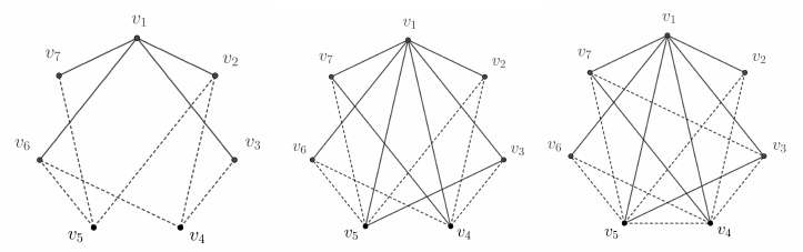
Proof. Due to Lemma 4, we need only show that \(\downarrow K_6\subseteq \langle K_{2,3}-e\rangle\cup \langle K_3\rangle\). So, consider the following four red-blue colorings of the edges of \(K_6\):
\(G_{r_1}\cong K_{2,4}+uv\), \(G_{b_1}\cong K_4\)
\(G_{r_2}\cong K_{1,5}\), \(G_{b_2}\cong K_{5}\)
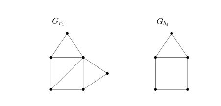
\(G_{r_3}\cong K_{3,3}\), \(G_{b_3}\cong K_3\cup K_3\)
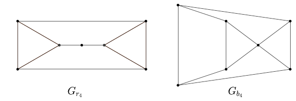
See Figure 2
We will show that the intersection of these four colorings is \(\langle K_{2,3}-e\rangle \cup \langle K_3\rangle\). First, using Example 1, we take the intersection of \(\mathcal{C}_1\) and \(\mathcal{C}_2\) to obtain the following. \[\left(\langle K_{2,4}+uv\rangle \cup \langle K_4\rangle \right)\cap \left(\langle K_{1,5}\rangle \cup \langle K_5\rangle \right)=\langle K_{2,3}+uv\rangle \cup \langle K_{1,5}\rangle \cup \langle K_4\rangle\]
Next, we take the intersection of \((1)\) and \(\mathcal{C}_3\) and use Observation 2 to reduce. \[\left(\langle K_{2,3}+uv\rangle \cup \langle K_{1,5}\rangle \cup \langle K_4\rangle \right)\cap \left(\langle K_{3,3}\rangle \cup \langle K_3\cup K_3\rangle \right)=\langle K_{2,3}\rangle \cup \langle K_3\rangle\] Finally, we find the intersection of \((2)\) and \(\mathcal{C}_4\) using Example 1 and Observation 4. Notice here that \(f_5\cong G_{r_4}\) and that \(G_{b_4}\subseteq G_{r_4}\). \[\begin{aligned} \left(\langle K_{2,3}\rangle \cup \langle K_3\rangle \right)\cap \left(\langle G_{r_4}\rangle \cup \langle G_{b_4}\rangle \right)&= \left(\langle K_{2,3}\rangle \cup \langle K_3\rangle \right)\cap \langle G_{r_4}\rangle \\ &=\langle K_{2,3}-e\rangle \cup \langle K_3\rangle \end{aligned}\]
Hence, \(\downarrow K_6\subseteq \langle K_{2,3}-e\rangle \cup \langle K_3\rangle\) ◻
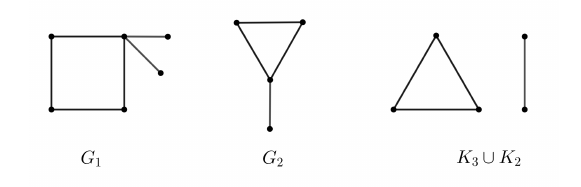
Next, we will show that the ideals generated by the three graphs in Figure 3 make up the down-arrow Ramsey set of \(K_7\).
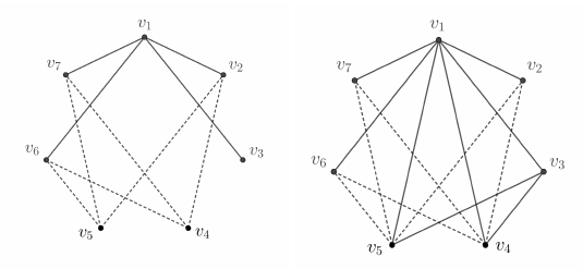
For ease of notation, we label the vertices of \(K_7\) from the set \(\{v_1, v_2, v_3,\) \(v_4, v_5, v_6, v_7\}\) for each of the following lemmas. Additionally, we will use solid line segments to represent red edges and dashed line segments to represent blue edges in the figures that follow.
Lemma 5. Let \(G_1\) be the graph obtained by adding two pendent edges to the same vertex of a four-cycle as in Figure 2. Then \(G_1 \in \ \downarrow K_7\).
Proof. Assume to the contrary that there exists a red-blue coloring \(\mathcal{C}\) of \(K_7\) that avoids a monochromatic \(G_1\). Since it is impossible to have a 3-regular graph of order 7, we know there must be a monochromatic \(K_{1, 4}\). Say there is a red subgraph isomorphic to \(K_{1,4}\) in the coloring \(\mathcal{C}\). Let the vertices of this subgraph be labeled \(v_1, v_2, v_3, v_6, v_7\) as shown in Figure 3. Consider another vertex, \(v_5\). Notice that \(v_5\) can be adjacent to at most one of the vertices \(v_2, v_3, v_6, v_7\) with a red edge, else a red \(G_1\) will be formed. Thus, \(v_5\) must be connected to at least three of \(v_2, v_3, v_6, v_7\) with blue edges. Without loss of generality, assume edges \(v_5v_2, v_5v_6, v_5v_7\) are blue. By the same argument, we know that \(v_4\) must also be adjacent to at least three of \(v_2, v_3, v_6, v_7\) with blue edges as well. We consider two cases.
Case 1. The edges \(v_4v_2, v_4v_6, v_4v_7\) are blue. There is a blue \(C_4\) formed, \((v_4, v_6, v_5, v_7, v_4)\). Since the edges \(v_2v_4\) and \(v_2v_5\) are also blue, then the following edges must be red to avoid a blue \(G_1\): \(v_1v_5\), \(v_3v_5\), \(v_1v_4\), \(v_1v_5\). However, this produces a red \(G_1\).
Case 2: The edges \(v_4v_2, v_4v_3, v_4v_6\) are blue. Again, we have formed a blue \(C_4\), \((v_2, v_4, v_6, v_5, v_2)\). Since the edges \(v_5v_7\) and \(v_3v_4\) are also blue, then the following edges need to be red: \(v_1v_4\), \(v_4v_7\), \(v_1v_5\), \(v_3v_5\).
Notice that if either are red, then the edges \(v_4v_5\) and \(v_3v_7\) would form a red \(G_1\). Thus, they must both be blue. However, if they are both blue, then there will be a blue \(G_1\).
Thus, no red-blue coloring of the edges of \(K_7\) that avoids a monochromatic \(G_1\) exists. ◻
Lemma 6. Let \(G_2\) be a triangle with a pendent edge as in Figure 3. Then \(G_2 \in \ \downarrow K_7\).
Proof. Assume to the contrary that there exists a red-blue coloring \(\mathcal{C}\) of the edges of \(K_7\) that avoids a monochromatic \(G_2\). Since the Ramsey number \(R(K_3, K_3)=6\), we know that there must be a monochromatic triangle in \(\mathcal{C}\). Assume without loss of generality that there is a red triangle, with vertices \(v_1\), \(v_2\), and \(v_3\). Since \(\mathcal{C}\) avoids a red \(G_2\), then all edges between \(\{v_1, v_2, v_3\}\) and \(\{v_4, v_5, v_6, v_7\}\) must be blue. Furthermore, all edges between the vertices in \(\{v_4, v_5, v_6, v_7\}\) will be red, else there will be a blue \(G_2\). However, this then forms a red \(K_4\), which clearly has a red \(G_2\) as a subgraph. Hence, all red-blue colorings of the edges of \(K_7\) must have a monochromatic \(G_2\). ◻
Lemma 7. \(K_3 \cup K_2 \in \ \downarrow K_7\).
Proof. Again, let’s assume that there exists a red-blue coloring \(\mathcal{C}\) of the edges of \(K_7\) that avoids a monochromatic \(K_3 \cup K_2\). Since there must be a monochromatic triangle, let’s assume that it is red and it has vertices labeled \(v_1\), \(v_2\), and \(v_3\). This time, all edges between the vertices in the set \(\{v_4, v_5, v_6, v_7\}\) must be blue to avoid a red \(K_3 \cup K_2\). This creates several blue triangles, one of which is formed between \(v_4\), \(v_5\), and \(v_6\). Thus, the edges \(v_1v_7\), \(v_2v_7\), and \(v_3v_7\) must be red. Similarly, \(v_5\), \(v_6\), and \(v_7\) form a blue triangle, so the edges \(v_1v_4\), \(v_2v_4\), and \(v_3v_4\) must also be red. However, this forces a red \(K_3 \cup K_2\). ◻
The above lemmas show that \(\langle G_1 \rangle \cup \langle G_2 \rangle \cup \langle K_3 \cup K_2 \rangle \subseteq \ \downarrow K_7\). Refer to the graphs \(G_3\) and \(G_4\) as depicted in Figure 7 in the following proof to show the reverse inclusion.
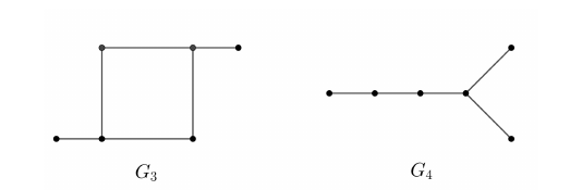
Theorem 11. The down-arrow Ramsey set \(\downarrow K_7=\langle G_1 \rangle \cup \langle G_2 \rangle \cup \langle K_3 \cup K_2 \rangle\).
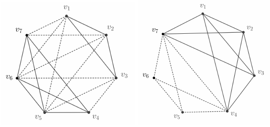
Proof. Consider the following five colorings of \(K_7\):
\(G_{r_1}\cong K_{2,5}+uv\), \(G_{b_1} \cong K_5\)
\(G_{r_2}\cong K_{1,6}\), \(G_{b_2} \cong K_6\)
\(G_{r_3}\cong K_3\cup K_4\), \(G_{b_3} \cong K_{3,4}\)
See Figure 8.
\(G_{r_5}\cong K_{3,3}\), \(G_{b_5}\cong \overline{K_{3,3}}\)
We now determine the intersection of these colorings by following Example 1 and Observation 2. First, we compute the intersection of colorings \(\mathcal{C}_1\) and \(\mathcal{C}_2\). \[\mathcal{C}_1\cap\mathcal{C}_2=\langle K_{1,6}\rangle\cup\langle K_5\rangle \cup \langle K_{2,4}+uv\rangle \tag{1}\] We now find the intersection of \((1)\) and \(\mathcal{C}_3\). The relevant intersections are computed below.
\(\langle K_{2,4}+uv\rangle \cap \langle K_3\cup K_4\rangle =\langle K_{4}-e\rangle \cup \langle K_2\cup K_{1,3}\rangle\)
\(\langle K_{2,4}+uv\rangle \cap \langle K_{3,4}\rangle = \langle G_2\rangle \cup \langle K_{2,4}\rangle\)
\(\langle K_{1,6}\rangle \cap \langle K_3\cup K_4\rangle =\langle K_{1,3}\rangle\)
\(\langle K_{1,6}\rangle \cap \langle K_{3,4}\rangle =\langle K_{1,4}\rangle\)
\(\langle K_5\rangle \cap \langle K_3\cup K_4\rangle =\langle K_4\rangle \cup \langle K_3\cup K_2\rangle\)
Hence, we have the following intersection. \[\left(\langle K_{1,6}\rangle\cup\langle K_5\rangle \cup \langle K_{2,4}+uv\rangle\right)\cap \mathcal{C}_3=\langle K_4\rangle \cup \langle K_3\cup K_2\rangle \cup \langle G_2\rangle \cup \langle K_{2,4}\rangle \tag{2}\] Now we take (2) and intersect with \(\mathcal{C}_4\) after noting the following intersections.
\(\left(\langle K_3\cup K_2\rangle \cup \langle G_2\rangle \right)\cap \left(\langle G_{r_4}\rangle \cup \langle G_{b_4}\rangle \right)=\langle K_3\cup K_2\rangle \cup \langle G_2\rangle\)
\(\langle K_4\rangle \cap \left(\langle G_{r_4}\rangle \cup \langle G_{b_4}\rangle \right)=\langle C_4\rangle \cup \langle G_2\rangle\)
\(\langle K_{2,4}\rangle \cap \left(\langle G_{r_4}\rangle \cup \langle G_{b_4}\rangle \right)=\langle G_1\rangle \cup \langle G_3\rangle\)
The intersection follows. \[\left(\langle K_4\rangle \cup \langle K_3\cup K_2\rangle \cup \langle G_2\rangle \cup \langle K_{2,4}\rangle\right)\cap \mathcal{C}_4=\langle G_1\rangle\cup \langle G_3\rangle \cup \langle K_3\cup K_2\rangle \cup \langle G_2\rangle \tag{3}\] Finally, we take the intersection of (3) and \(\mathcal{C}_5\).
\(\langle K_{3,3}\rangle \cap \langle G_1\rangle =\langle K_{2,3}-e\rangle\cup \langle 2P_3\rangle\)
\(\langle K_{3,3}\rangle \cap \langle G_3\rangle = \langle K_{2,3}-e\rangle \cup \langle 2P_3\rangle\)
\(\langle K_{3,3}\rangle \cap \langle K_3\cup K_2\rangle =\langle P_3\cup K_2\rangle\)
\(\langle K_{3,3}\rangle \cap \langle G_2\rangle =\langle K_{1,3}\rangle \cup \langle P_4\rangle\)
\(\langle G_{b_5}\rangle \cap \langle G_2\rangle =\langle G_2\rangle\)
\(\langle G_{b_5}\rangle \cap \langle K_3\cup K_2\rangle =\langle K_3\cup K_2\rangle\)
\(\langle G_{b_5}\rangle \cap \langle G_3\rangle =\langle K_{2,3}-e\rangle \cup \langle G_4\rangle\)
\(\langle G_{b_5}\rangle \cap \langle G_1\rangle =\langle G_1\rangle\)
Thus, we have our final intersection. \[\left(\langle G_1\rangle\cup \langle G_3\rangle \cup \langle K_3\cup K_2\rangle \cup \langle G_2\rangle\right)\cap \mathcal{C}_5=\langle G_1\rangle \cup \langle G_2\rangle \cup \langle K_3\cup K_2\rangle \tag{4}\] Hence, \(\downarrow K_7 \subseteq (4)\), and we have \(\downarrow K_7 = \langle G_1\rangle \cup \langle G_2\rangle \cup \langle K_3\cup K_2\rangle\). ◻
There are a number of directions that research in this topic can go. The most obvious is to determine \(\downarrow K_n\) for larger values of \(n\). Other developments in this area may arise from one of the following pursuits.
Develop new computational methods for computing intersections of ideals.
Consider multi-color Ramsey numbers.
Study minimal sets of colorings needed to determine a down-arrow Ramsey set.
Let’s consider this last suggestion in more detail. By Proposition 1, we know there exists a finite set of colorings which, when combined properly through graph ideal intersections, give the down-arrow Ramsey set for any graph \(G\). However, it is not computationally feasible to compute the graph ideal intersections for all colorings of a graph. Hence, further research will be devoted to finding small sets of colorings that determine the down-arrow Ramsey set, that is, collections of colorings that satisfy the conclusion of Proposition 1. To this end, we define the following terminology. Let \(G\) be a nonempty graph of order \(n\ge 2\). A set of colorings \(\mathcal{H}\) satisfying the conclusion of Proposition 1 will be referred to as a Ramsey elimination set. A Ramsey elimination set of minimum cardinality is called a minimum Ramsey elimination set. The cardinality of a minimum Ramsey elimination for \(G\) is called the Ramsey elimination number of \(G\) and is denoted \(Re(G)\).
From this definition, there are several problems one can investigate. We identify perhaps the most fruitful here.
Problem 1. For a given graph \(G\), find properties that a minimum Ramsey elimination set must possess. Determine if a set of colorings is a Ramsey elimination set for \(G\) without knowing \(\downarrow G\) a priori.
A solution or partial solution to the previous problem will be useful in reducing the field of possible sets of colorings. It may then be computationally feasible to determine the graph ideal intersections. Some work has been done to attack this problem, in particular, we compute \(Re(G)\) and give a minimum Ramsey elimination set for some of the complete graphs in this paper.
Proposition 7. The Ramsey elimination number of \(K_3\) is 1.
Proof. We know that \(\downarrow K_3=\langle P_3\rangle.\) Take the set of colorings \(\mathcal{H}=\{(P_3, K_2)\}\), and observe that \(\langle P_3\rangle \cup \langle K_2\rangle =\langle P_3\rangle\). Since \(Re(G)\ge 1\) for all non-empty graphs \(G\), it follows that \(Re(K_3)=1\), and a minimum Ramsey elimination set is given by \(\mathcal{H}=\{(P_3,K_2)\}\). ◻
Proposition 8. The Ramsey elimination number of \(K_4\) is 2.
Proof. We know that \(\downarrow K_4=\langle P_3\rangle\). In Proposition 5 it is verified that \(\mathcal{H}=\{(K_3, K_{1,3}),(C_4,2K_2)\}\) is a Ramsey elimination set. It remains to be seen that this is a minimum Ramsey elimination set. Suppose that there exists a graph \(H\) for which \(\downarrow K_4=\langle H\rangle \cup \langle \overline{H}\rangle\), then we would have that \(\langle P_3\rangle =\langle H\rangle \cap \langle \overline{H}\rangle\). However, since \(K_4\) has \(6\) edges, it must be that \(|E(H)|+|E(\overline{H})|=6\). Hence, either \(|E(H)|\ge 3\) or \(|E(\overline{H})|\ge 3\). that is, there exists graphs in \(\langle H\rangle \cup \langle \overline{H}\rangle\) with \(3\) edges. However, \(P_3\) has only two edges, so this is impossible. ◻
The technique used in the last example can be generalized.
Proposition 9. Let \(G\) be a graph of order \(n\) and size \(m\). If for each \(H\in \downarrow G\) we have \(|E(H)|<\frac{m}{2}\), then \(Re(G)\ge 2\).
Proof. Suppose \(Re(G)=1\), then there exists \(H\) such that \(\downarrow G=\langle H\rangle \cup \langle \overline{H}\rangle\). Since \(|E(H)|+|E(\overline{H})|=m\), it must be that either \(|E(H)|\ge \frac{m}{2}\) or \(E(\overline{H})\ge \frac{m}{2}\). Hence, there is some graph in \(\downarrow G\) with at least \(\frac{m}{2}\) edges. ◻
Proposition 10. The Ramsey elimination number of \(K_5\) is \(2\).
Proof. We know that \(\downarrow K_5=\langle P_4\rangle\). In Proposition 6 it is verified that \(\mathcal{H}=\{(C_5,C_5),(K_4,K_{1,4})\}\) is a Ramsey elimination set. Furthermore, since \(P_4\) generates \(\downarrow K_5\) and has only \(3\) edges, it follows by Proposition 9 that \(Re(K_5)=2\) and \(\mathcal{H}\) is a minimum Ramsey elimination set. ◻
In addition to investigating the problems posed above in relation to Ramsey elimination sets, further work can be done on finding specific down-arrow Ramsey sets that are not included or finished in this paper. For example, we will continue to work on describing the down-arrow Ramsey set for all complete bipartite graphs \(K_{s,t}\) for \(t\geq 1\) and \(s\geq3\). Additionally, determining the down-arrow Ramsey sets for larger complete graphs is an alluring topic due to its connection to traditional Ramsey Theory. In this case, we believe that further research into Ramsey elimination sets and intersections of graph ideals will prove crucial in this effort.
We greatly appreciate the valuable suggestions made by Jamie Hallas that resulted in an improved paper.