
A graph \(G=(V,E)\) is a connected, undirected, and simple graph with the vertex set \(V(G)\) and the edge set \(E(G)\). The degree or valency of a vertex \(v\) in graph \(G\ \)is defined as the number of edges that connect to \(v\), and it is represented as \(\mathrm{deg}\mathrm{}\mathrm{(}v\mathrm{)}\). The minimum degree of a graph \(G\) is denoted by \(\delta \mathrm{(}G\mathrm{)}\) while the maximum degree is denoted by \(\mathrm{\Delta }\mathrm{(}G\mathrm{)}\). Similarly tree is also defined as an undirected graph in which every two vertices are connected by exactly one path and to be more precise any acyclic connected graph is a tree. This article deals with vertex k-labeling of two types of trees namely star \(S_{m,n}\) and banana tree \({BT}_{m,n}\) by using the combinatorial properties of graphs that satisfy on trees as well in the context of labeling.
Graph labeling is the process of assigning integers to the vertices or edges or both, of a graph by satisfying certain condition(s). In 1988, Chartrand et al. [1] introduced the concept of edge k-labeling, where edges in a graph are assigned labels with the condition that the weights of vertices must be unique. In 2014, Ahmad et al. [2] introduced vertex \(k\)–labeling also known as edge irregular \(k\)–labeling as an extension of Chartrand’s work. According to this definition, vertices are labeled in a way that weights of all edges remain unique, i.e., for any distinct pair of edges \(e\) and \(e'\) weights \({wt}_{\emptyset }(e)\neq {wt}_{\emptyset }(e')\). While the weight for any edge is calculated by adding the labels of its adjacent vertices \({wt}_{\emptyset }\left(e\right)=\emptyset \left(x\right)+\emptyset \left(xy\right)+\emptyset (y)\). The edge irregularity strength of a graph \(G\), denoted as \(es(G)\), represents the minimum value of \(k\) for which \(G\) can have an edge irregular \(k\)–labeling. Theorem 1 of [2], established the lower bound for the edge irregularity strength of any graph \(G\). Meanwhile an upper bound or tightness of \(es\left(G\right)\ \)for different graph families is proved in many papers [1,3-9].
Theorem 1. [2] Let \(G=(V,E)\) be a simple graph with maximum degree \(\Delta \ =\Delta (G)\). Then \[\label{GrindEQ__1_} es\left(G\right)\ge max\ \left\{\left\lceil \frac{\left|E\left(G\right)+1\right|}{2}\right\rceil ,\Delta (G)\right\}\tag{1}\]
A tree is a type of undirected, connected graph without any cycles or loops. Tree one of the important non-linear discrete structure heavily used in computer applications [10]. Tree are classified in so many ways, a common category is rooted tree where one vertex is designated as a root (at level-0) and every edge is directed away from the root towards other vertices that are placed in successive levels through a unique path. An \(m\)-ary tree is defined as a rooted tree where each internal vertex has at most m children [11]. Rooted trees are important in computer science, as their hierarchical structure is suitable in file-systems, efficient access to large data sets, data encoding and so many other Algorithms. The prominent uses of trees include Huffman coding and Tries [12], which are employed to construct efficient codes for data transmission and storage. Tree algorithms are used in workflow management and path determination in networks.
Interdisciplinary research among discrete mathematics and computer science has evolved many applications by implementing graphs and tree algorithms such as data representation, network analysis and optimization, searching and traversal, data organization and retrieval, machine learning, bioinformatics, linguistics theory and cryptology. Algorithms solve many problems, whereas other mathematical solutions are very complex or impossible. In 2018, Asim et al. [13] used algorithmic approach for computing a tight upper-bound for vertex \(k\)-labeling of complete graphs as \(es\left(K_n\right)\mathrm{=}{Elog}_2\mathrm{V}\) in comparison to previously known loose upper-bound as \(es\left(K_n\right)\mathrm{=}F_n\).The \(F_n\) of Fibonacci numbers be defined by the recurrence relation \(F_n=F_{n-1}+F_{n-2}\ \) [13]. Ahmad et al. [11] worked on a computer-based experiment for the vertex \(k\)-labeling of the \(m\)–ary tree \(T_{m,h}\). They performed experiments on complete binary and ternary tree and finally devised general algorithm for vertex k-labeling on complete \(m\)–ary tree as \(es\left(T_{m,h}\right)=\left[\frac{v}{2}\right]\) for any height h. Asim et al. [14] computed the vertex \(k\)-labeling of circulant graphs using algorithmic approach. They used decomposition on complete graphs, by deleting factors or Hamiltonian cycles to extract circulant graphs as subgraphs. Recently, Ahmad et al. [7] computed the edge irregularity strength of bipartite graphs and wheel-related graphs using an algorithmic approach. Using the experimental results they provided an upper-bound for edge irregularity strength of a complete bipartite graph \(K_{m,n}\).
This section introduces empirical techniques employed to reach conclusions based on the observations made through extensive literature review, and mathematical properties of graph labeling are studied to formulate specific claims on edge irregular k-labeling in star graphs and banana trees. In the research instrumentation phase inductive technique is adopted to shape the objects of study from specific to general by comparing the computer-generated results with mathematical theorems. This involved developing and implementing algorithms on a computer, as well as collecting and analyzing empirical data for various instances of amalgamated star and banana trees. Invariants of the trees for both problems are inserted as input of the algorithms systematically to plot the curve of results to compare with lower-bounds. The primary objective is to ensure the correctness of algorithms to validate the k-labeling using double inequality among upper and lower bounds.
Both algorithms are designed using iterative approach to compute the results efficiently. Algorithms solved the problems repeatedly in a step-by-step manner which enabled systematic and efficient computations. The algorithms are implemented on computer at large-scale experiment by variating the values of \(m\) and \(n\) as different treatments of the experiment. From the perspective of computational complexity, efficiencies of the algorithms are analyzed in terms of scalability, time complexity, space complexity. All these dependencies like availability of the algorithms and computational cost that are not present in case of mathematical proofs for labeling any graph or tree, it is practical to solve such problems that are still open due to absence of labeling patterns and unavailability of formulae.[15-19]
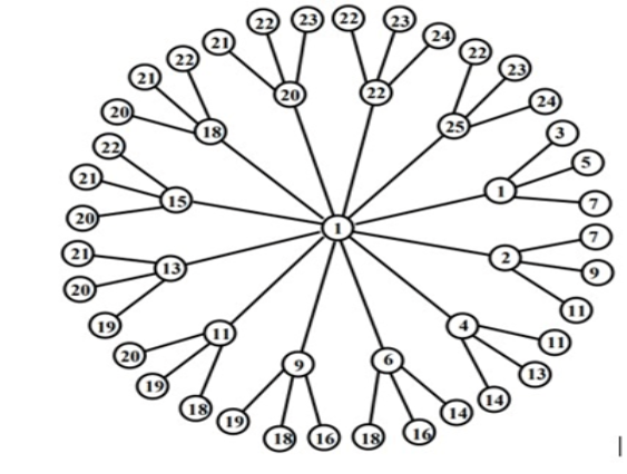
Consider \(m\) homogenous disjoint stars of any order \(n\), for \(n\ge 3\). The amalgamation of stars can be obtained by joining the central vertex of each star with an additional vertex, denoted by \(S_{m,n}\). The example of a homogenous amalgamated star graph \(S_{12,4}\) is shown in Figure 1, where \(m\) represents the degree of additional vertex and \(n\) represents the degree of a central vertex of each star. This problem is an extension or generalization of Asim et al. [20] work where they mathematically proved that the \(es(S_{m,n})\) for any value of \(m\) but the value of \(n\le 3\). This article provides the algorithmic solution of \(es(S_{m,n})\) for any value of \(m\ge 2\) and \(n\ge 3\).
Theorem 2. Let \(S_{m,n}\) be a homogenous amalgamated star graph with \(m\ge 2\) and \(n\ge 3\), then \[es(S_{m,n})\ge \left\lceil \frac{|V|}{2}\right\rceil .\]
Proof. The maximum degree of a homogenous amalgamated star graph \(S_{m,n}\) may be \(m\) or \(n\). From Theorem 1, \(es(S_{m,n})\ge \left\lceil \frac{(m\ast n)+1}{2}\right\rceil\). For converse inequality, we prove the \(es(S_{m,n})\) and an algorithm is designed which assigns the labels to the vertices by ensuring the condition that edge weights do not repeat. Let \(\left|V\right|\) be the order of \(S_{m,n}\) that is \((m\ast n)+1=|V|\). The functionality of the algorithm is explained below:
This algorithm comprises on four steps to compute the labels of \(S_{m,n}\) graph. The vertex with degree m, known as the centroid vertex, is labeled as 1. Subsequently, the immediate vertices connected to the centroid vertex, which can be considered first-level vertices, are assigned labels using a formula based on the difference. This difference formula is calculated based on the values of \(m,n\) and \(\left|V\right|\). The labels of the first-level vertices are stored in an array, along with their corresponding edge weights. In the same way, to assign the label to pendent vertices (second-level vertices), previously used edge weights are excluded to maintain uniqueness. This provides \(es(S_{m,n})\le \left\lceil \frac{m*n+1}{2}\right\rceil\). ◻
Input: Two positive integers \(n\) and \(m\), where \(m, n \geq 2\)
Output: Labels of vertices \(\{1, 2, \dots, k\}\) stored in arrays L1 and L2.
\(V = m * n + 1\)
\(Diff = \left\lfloor \frac{\lceil |V| / 2\rceil}{m-1} \right\rfloor\)
\(L0 = 1\)
\(L1[1-3][1] = 0, 1, 2\)
for \(i=2\) to m do
\(L1[1][i] = L1[1][i – 1] + Diff\)
\(L1[2][i] = \lfloor L1[1][i] \rfloor\)
\(L1[3][i] = L1[2][i] + 1\)
end for
\(L1[3][m + 1] = NIL\)
\(h, j = 1, 2\)
for \(wt=3\) to V do
if \(wt≠L1[3][j]\) then
\(L2[1][h] = wt\)
\(h = h + 1\)
else
\(j = j + 1\)and if
and for
Computational complexity or precisely time complexity T(n) of an algorithm means quantification of time taken by an algorithm to produce desired output from given input. Where T is time (dependent factor) and n (independent factor) is amount of data to be handle. In our case m and n are two invariants of the trees that defines the structure of star tree, how many vertices and how big and difficult the problem can be. In the algorithm there are some atomic statements that always cost T(1) but iterations in the algorithm actually determines the growth of function for T(m,n). The loop given on line 5-9 cost T(m), similarly the loop given on line 12-21 cost T(V). Hence the total cost of the algorithm can be represented using the expression \(m+V\). The dominant factor in the time complexity is \(V\) so on big \(O\) notation as the order of growth of function, it can be expressed as \(T(m,V)=O\left(V\right)\).
Algorithm follows iteration as design architecture and mainly rely on two simple loops. Two 2D-Arrays, \(L\mathrm{1}\) and \(L\mathrm{2}\) are used to store the labels and edge weights of level-1 and level-2 vertices separately. Centroid vertex and one of the incident vertices to centroid vertex is labeled as 1 and stored in the array as seed value. Then using the difference formula \(Diff = \left\lfloor \frac{\lceil |V| / 2\rceil}{m-1} \right\rfloor \)all other labels are computed in first level. For labeling pendant vertices (the second level), scheme is reversely applied as weights are given to the edges first and then labels are computed by subtracting the label of parent from the edge-weight. For this purpose and an efficient expression is devised as written on line 15. In this whole process it is asserted that the edge weights remain unique and for this purpose if condition is given on line 13.
Results of Algorithm-1 are shown in Table 1 as the upper bound, while the lower bound is mathematically calculated using Theorem 1. Both columns reflect the same values which means the algorithm is working perfectly and computing the correct labels. The fact that the mathematically derived lower bounds and the results from the algorithm match each other shows that the algorithm is working correctly and producing accurate labels. This proves that the algorithm is reliable and can be trusted to accurately compute the desired labels. This also proves that computation error is zero, as the algorithm produces the correct labeling without any errors.
| Input List | Calculated Values | |||
|---|---|---|---|---|
| \(m\) | \(n\) | \(V\) | Lower Bound \(\mathrm{\lceil }\)( \(\frac{V}{2}\) )\(\mathrm{\rceil }\) | Algorithmic Result \(k=es(S_{m,n})\) |
| 3 | 3 | 10 | 5 | 5 |
| 3 | 10 | 31 | 16 | 16 |
| 3 | 100 | 301 | 151 | 151 |
| 3 | 1000 | 3001 | 1501 | 1501 |
| 4 | 3 | 13 | 7 | 7 |
| 4 | 10 | 401 | 201 | 201 |
| 4 | 1000 | 4001 | 2001 | 2001 |
| 5 | 3 | 16 | 8 | 8 |
| 5 | 10 | 51 | 26 | 26 |
| 5 | 100 | 501 | 251 | 251 |
| 5 | 1000 | 5001 | 2501 | 2501 |
| 10 | 3 | 31 | 16 | 16 |
| 10 | 10 | 101 | 51 | 51 |
| 10 | 100 | 1001 | 501 | 501 |
| 10 | 1000 | 10001 | 5001 | 5001 |
| 100 | 3 | 301 | 151 | 151 |
| 100 | 100 | 10001 | 5001 | 5001 |
| 100 | 1000 | 100001 | 50001 | 50001 |
| 1000 | 3 | 3001 | 1501 | 1501 |
| 1000 | 10 | 10001 | 5001 | 5001 |
| 1000 | 100 | 100001 | 50001 | 50001 |
| 1000 | 1000 | 1000001 | 500001 | 500001 |
Let \(G_{\mathrm{1}},G_{\mathrm{2}},G_{\mathrm{3}}\mathrm{,\dots ,}G_m\) be a family of m homogenous disjoint stars with order \(n\). Let \(v\) be a new vertex and the tree obtained by joining \(v\) to one pendant vertex of each star is called a banana tree. In 2021, Ahmad [16] worked on even branches of banana trees and proved that even values of \(m\) banana tree admit the edge irregular k\(\mathrm{-}\)labeling, while he left two open problems as given below:
Problem 1. [21] Let \(G\cong BT(n_1,n_2,n_3,\dots ,nm)\) be a banana tree. For \(n_1=m_2=\dots =nm=n\ge 3\) and \(m\ge 5\) odd, the graph \(G\) admits an edge irregular \(\left\lceil \frac{m\left(n+1\right)+1}{2}\right\rceil\) \(\mathrm{-}\) labeling.
Problem 2. [21] Let \(H\cong BT(n_1,n_2,n_3,\dots ,nm)\) be a tree. For \(n_1=m_2=\dots =nm=n\ge 3\) and \(m\ge 3\) odd, the graph \(H\) admits an edge irregular \(\left\lceil \frac{m\left(n+1\right)+2}{2}\right\rceil\) \(\mathrm{-}\) labeling.
A comprehensively designed algorithm, using an iterative approach, has been implemented to cover the labeling of all classes of banana trees. An iterative approach helps in solving complex problems in a step-by-step manner. The algorithm is implemented on a computer, and a large-scale experiment is conducted for different values of \(m\) and . The results of the algorithms are shown in Table 2. Let \({BT}_{m,n}\) be a symmetry banana tree having \(m\) stars and \(n\) is the order of each star. Let \(\left|V\right|\) be the order of \({BT}_{m,n}\). The value of \(m\) and the value of \(n\) should be greater than 2. Note that \(m\) is the number of vertices attached to the root and \(\mathrm{(}n\mathrm{-}\mathrm{2)}\) is the number of leaves of each star. The banana tree \({BT}_{\mathrm{4,7}}\) is represented in Figure 2 as an example.
| Input List | Calculated Values | |||
|---|---|---|---|---|
| m | n | V | Lower Bound \(\mathrm{\lceil }\)( \(\frac{V}{2}\) )\(\mathrm{\rceil }\) | Algorithmic Result \(k=es({BT}_{m,n})\) |
| 3 | 3 | 10 | 5 | 5 |
| 3 | 4 | 13 | 7 | 7 |
| 3 | 10 | 31 | 16 | 16 |
| 3 | 100 | 301 | 151 | 151 |
| 3 | 1000 | 3001 | 1501 | 1501 |
| 5 | 3 | 16 | 8 | 8 |
| 5 | 4 | 21 | 11 | 11 |
| 5 | 5 | 26 | 13 | 13 |
| 5 | 10 | 51 | 26 | 26 |
| 5 | 100 | 501 | 251 | 251 |
| 5 | 1000 | 5001 | 2501 | 2501 |
| 10 | 3 | 31 | 16 | 16 |
| 10 | 6 | 61 | 31 | 31 |
| 10 | 10 | 101 | 51 | 51 |
| 10 | 100 | 1001 | 501 | 501 |
| 10 | 999 | 9991 | 4996 | 4996 |
| 10 | 1000 | 10001 | 5001 | 5001 |
| 100 | 3 | 301 | 151 | 151 |
| 100 | 10 | 1001 | 501 | 501 |
| 100 | 100 | 10001 | 5001 | 5001 |
| 100 | 1000 | 100001 | 50001 | 50001 |
| 1000 | 3 | 3001 | 1501 | 1501 |
| 1000 | 10 | 10001 | 5001 | 5001 |
| 1000 | 100 | 100001 | 50001 | 50001 |
| 1000 | 1000 | 1000001 | 500001 | 500001 |
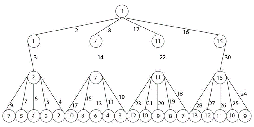
The banana tree \({BT}_{4,7}\) comprises 4 stars, each with an order of 7, denoted as \(m\) = 4 and \(n\ \)= 7. The total number of vertices \(\left(V\right)\) is determined by calculating \(V=m\ \times n+1\), resulting in \(V\) = 29. To find the value of \(K\), the ceiling function \(\left\lceil \frac{V}{2}\right\rceil\) is applied, yielding \(\left\lceil \frac{29}{2}\right\rceil\) \(=15\). Therefore, \(K\) = 15. Next, the distance formula is calculated as \(=\frac{K}{m}\) , equivalent to \(\frac{15}{4}\) = = 3.75. Let’s begin by assigning label 1 to the root vertex, and then proceed to assign labels to the vertices in the first level. The label 1 is assigned to the leftmost vertex. Then, the difference is added twice to the neighboring vertex, resulting in 7.5. However, only the integer value, 7, is considered while ignoring the decimal point. The label of the third vertex is indeed obtained by adding the difference to the previous value, resulting in 7.5 + 3.75 = 11.25, and it assigns the label as 11. Similarly, the label of the fourth vertex is calculated as 11.25 + 3.75 = 15, and it it assigns the label as 15.
Once all vertices have received labels, the edge weight is calculated by summing the labels of the connected vertices. These edges are stored in a dataset to prevent repetition. Moving to the next level of vertices, the leftmost vertex is assigned the label 2, while the remaining vertices inherit the label of their parent vertex. Starting from the leftmost vertex, the labels progress as 2, 7, 11, and 15 from left to right. The edge weight for all vertices in level 2 is calculated following the same process.
In the last level of vertices, starting from the leftmost side, the minimum possible labels are determined by calculating the difference from the parent vertex label to itself, ensuring the establishment of unique edge weights between them. The dataset stores all the unique edge weights, which are calculated from 2 to V+1, equivalent to 2 to 30 while ensuring no repetition of edge weights between any two vertices. This process continues as it moves to the next star, progressing towards the rightmost side until the last star is reached.
Input: Two positive integers \(n\) and \(m\), with \(m, n \ge 2\)
Output: Labels of vertices \(\{1, 2, \ldots, k\}\) stored in arrays L1 and L2.
\(V \gets m \ast n + 1\)
\(\textit{Diff} \gets \left\lceil \frac{|V|}{2} \right\rceil\)
\(\textit{L}0 \gets 1\)
\(\textit{L}1[1\ldots 5][1] \gets \textit{Diff}, 1, 2, 2, 3\)
for \(i=2\) to m do
\(\textit{L}1[1][i] \gets \textit{L}1[1][i – 1] + \textit{Diff}\)
\(\textit{L}1[2][i] \gets \left\lfloor L1[1][i] \right\rfloor\)
\(\textit{L}1[3][i] \gets \textit{L}1[2][i] + 1\)
\(\textit{L}1[4][i] \gets \textit{L}1[2][i] + 1\)
\(\textit{L}1[5][i] \gets \textit{L}1[2][i] + L1[2][i]\)
end for
\(\textit{L}1[3][m+1] = \textit{NIL}\)
\(j, h, q \gets 2, 1, 2\)
for \(wt=2\) to \(V-1\) do
if \(wt≠L1[4][j]\) and \(wt≠L1[5][q]\) then
\(\textit{L}2[1][h] \gets \textit{wt}\)
\(\textit{L}2[2][h] \gets \textit{wt} – L1[3]\left[ \left\lfloor \frac{h + (n – 3)}{(n-2)} \right\rfloor \right]\)
\(h = h + 1\)
else
if \(wt≠L1[4][j]\) then
\(j = j + 1\)
else
\(q = q + 1\)
end if
end if
end for
The computational complexity of an algorithm is denoted by \(T(n)\), where \(T\) represents the time (dependent factor), and \(n\) is the input size (independent factor). In the “Banana Tree” algorithm, denoted as \(BT_{(m,n)}\), \(m\) represents the number of stars, and \(n\) is the order of each star in the tree. The algorithm includes some atomic statements that always incur a constant cost of \(T\eqref{GrindEQ__1_}\). However, the growth of the function for \(T(n)\) is determined by the iterations in the algorithm. The iterations involve two ’for loops,’ from line 5 to 11 and from line 14 to 27. The first iteration’s cost is \(m\), and the second iteration’s cost is \(V-3\), respectively. Thus, the total cost of the algorithm can be represented by the expression \(m+V-3\). The dominant factor in the time complexity is \(V\), so in Big O notation, it can be expressed as \(T\left(m,V\right)=O(V)\).
Algorithm follows iteration as design architecture and mainly rely on two simple loops. Two 2D-Arrays, \(L\mathrm{1}\) and \(L\mathrm{2}\) are used to store the labels and edge weights of level-1 and level-2 vertices separately. Root vertex and one of the left most incident vertices from the root vertex is labeled as 1 and stored in the array as seed value. Then using the difference formula \(Diff={{\frac{\left\lceil \left|\boldsymbol{V}\right|\right\rceil }{\boldsymbol{2}}}}\ \)all other labels are computed in first level. For the second level, the labels are computed similarly to the last level, except for the first vertex from the left side. The first vertex from the left side of the second level will receive a value obtained by adding 1 to the label of the corresponding vertex in the previous level. For labeling pendant vertices (the third level), scheme is reversely applied as weights are given to the edges first and then labels are computed by subtracting the label of parent from the edge-weight. For this purpose and an efficient expression is devised as written on line 17. In this whole process it is asserted that the edge weights remain unique and for this purpose ‘if ’condition is given on line 15.
Table 2 presents the results of Algorithm-2, representing the upper bound, while Theorem 1 is applied to mathematically calculate the lower bound. Both columns show the same values, indicating that the algorithm is working perfectly and has computed the correct labels. The fact that the mathematically derived lower bounds and the results from the algorithm match each other demonstrates the algorithm’s accuracy and correctness. This proves the reliability of the algorithm, as it can be trusted to accurately compute the desired labels. Furthermore, it is worth noting that there are no errors while computing the labels, which reinforces the algorithm’s precision. The consistent production of correct labeling without any errors adds to the confidence in the algorithm’s accuracy and reliability.
Through the implementation of iterative algorithms and the utilization of research methodologies, the accuracy and correctness of the labeling results have been established. The comparison of computer-generated results with the established mathematical known results, along with the validation of lower bounds, further confirms the effectiveness of the algorithmic approach in computing edge irregular \(K\)-labeling. To justify the correctness of the algorithmic approach, results are implemented on the computer and shown as tabular facts in Table 1 for \(es(S_{m,n})\) and in Table 2 for \(es({BT}_{m,n})\). These tables depict that both trees are tight for edge irregular \(\left\lceil \frac{\left|V\right|}{2}\right\rceil\) -labeling. This statement can be written mathematically by combining the results of the experiment and Theorem 1 in the form of double inequality. For amalgamated star graph \(S_{m,n}\), we have \(\left\lceil \frac{\left|V\right|}{2}\right\rceil\) \(\mathrm{\le}\) \(es(S_{m,n})\) \(\mathrm{\le}\) \(\left\lceil \frac{\left|V\right|}{2}\right\rceil\) and similarly for banana tree \({BT}_{m,n}\), we have \(\left\lceil \frac{\left|V\right|}{2}\right\rceil \ \)\(\mathrm{\le}\)\(\ es({BT}_{m,n})\) \(\mathrm{\le}\) \(\left\lceil \frac{\left|V\right|}{2}\right\rceil\). In the future, these algorithms can be customized for other types of trees that maybe more complex, irregular in shapes, temporal in nature to use in them in the applications like decision trees and knowledge trees.