The Domination Number of   $C_n\square P_m$ for $n\equiv 2\pmod{5}$

Guichard, David R.

doi:10.61091/jcmcc120-040

Abstract

1. Introduction
2. Lower Bound
3. The Algorithm
4. Upper Bound
5. Summary

References

Journal of Combinatorial Mathematics and Combinatorial Computing

Volume 120
Pages: 435-443

Research article

The Domination Number of $C_{n} P_{m}$ for $n \equiv 2 (\mod 5)$

^¹

¹Whitman College, 345 Boyer Ave, Walla Walla, WA 99362

Received: 02/03/2020
Accepted: 24/05/2021

Copyright Link
License

Abstract

We use a dynamic programming algorithm to establish a new lower bound on the domination number of complete cylindrical grid graphs of the form $C_{n} P_{m}$ , that is, the Cartesian product of a path and a cycle, when $n \equiv 2 (\mod 5)$ , and we establish a new upper bound equal to the lower bound, thus computing the exact domination number for these graphs.

Keywords: Dynamic programming algorithm, Grid graph, Domination number

1. Introduction

A set $S$ of vertices in a graph $G = (V, E)$ is called a dominating set if every vertex $v \in V$ is either in $S$ or adjacent to a vertex in $S$ . The domination number of $G$ , $γ (G)$ , is the minimum size of a dominating set.

Let $P_{m}$ denote the path on $m$ vertices and $C_{n}$ the cycle on $n$ vertices; the complete cylindrical grid graph or cylinder is the product $C_{n} P_{m}$ . That is, if we denote the vertices of $C_{n}$ by $u_{1}, u_{2}, \dots, u_{n}$ and the vertices of $P_{m}$ by $w_{1}, \dots, w_{m}$ , then $C_{n} P_{m}$ is the graph with vertices $v_{i, j}$ , $1 \leq i \leq n$ , $1 \leq j \leq m$ , and $v_{i, j}$ adjacent to $v_{k, l}$ if $i = k$ and $w_{j}$ is adjacent to $w_{l}$ or if $j = l$ and $u_{i}$ is adjacent to $u_{k}$ . It will be useful to think of this graph as $P_{n} P_{m}$ , with the edge paths of length $m$ glued together, that is, connected with new edges. We assume throughout that $m \geq 2$ and $n \geq 3$ .

P. Pavlič and J. Žerovnik [1] established upper bounds for the domination number of $C_{n} P_{m}$ , and José Juan Carreño et al. [2] established non-trivial lower bounds. For $n \equiv 0 (\mod 5)$ the bounds agree, so the domination number is known exactly. In [3], we improved the lower bounds, except of course in the case that $n \equiv 0 (\mod 5)$ . Using the same techniques, we improve the lower bound slightly when $n \equiv 2 (\mod 5)$ , and we show that this value is the true domination number by also slightly improving the known upper bound.

2. Lower Bound

We summarize the technique for computing a lower bound; details are in [3]. A vertex in $C_{n} P_{m}$ dominates at most five vertices, including itself, so certainly $γ (C_{n} P_{m}) \geq n m / 5$ . If we could keep the sets dominated by individual vertices from overlapping, we could get a dominating set with approximately $n m / 5$ vertices, and indeed we can arrange this for much of the graph, with the exception of the “edges”, that is, the two copies of $C_{n}$ in which the vertices have only 3 neighbors, and except when $n \equiv 0 (\mod 5)$ , we run into some trouble where the edge paths of $P_{n} P_{m}$ are connected to form $C_{n} P_{m}$ .

Suppose $S$ is a subset of the vertices of $C_{n} P_{m}$ . Let $N [S]$ be the set of vertices that are either in $S$ or adjacent to a member of $S$ , that is, the vertices dominated by $S$ . Define the wasted domination of $S$ as $w (S) = 5 | S | - | N [S] |$ , that is, the number of vertices we could dominate with $| S |$ vertices in the best case, less the number actually dominated. When $S$ is a dominating set, $| N [S] | = m n$ , and if $w (S) \geq L$ then $| S | \geq (L + m n) / 5$ . Our goal now is to find a lower bound $L$ for $w (S)$ .

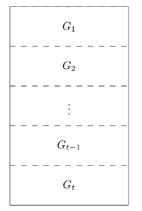
Suppose a cylinder $C_{n} P_{m}$ is partitioned into subgraphs as indicated in Figure 1, where each $G_{i}$ is a subgraph $C_{n} P_{m_{i}}$ . (We will refer to $G_{1}$ and $G_{t}$ as edge subgraphs, and the others as interior subgraphs.) Let $S$ be a dominating set for $G$ and $S_{i} = S \cap V (G_{i})$ . Then $\begin{matrix} (1) & w (S) \geq \sum_{i = 1}^{t} w (S_{i}) . \end{matrix}$ Note that in computing $w (S_{i})$ we consider $S_{i}$ to be a subset of $V (G)$ , not of $V (G_{i})$ (this affects the computation of $N [S_{i}]$ ). To verify the inequality, note that the following inequalities are equivalent: $\begin{aligned} w (S) & \geq \sum_{i = 1}^{t} w (S_{i}) \\ 5 | S | - | N [S] | & \geq \sum_{i = 1}^{t} (5 | S_{i} | - | N [S_{i}] |) \\ 5 | S | - | N [S] | & \geq \sum_{i = 1}^{t} 5 | S_{i} | - \sum_{i = 1}^{t} | N [S_{i}] | \\ | N [S] | & \leq \sum_{i = 1}^{t} | N [S_{i}] | . \end{aligned}$ The last inequality is satisfied, since each vertex in $N [S]$ is counted at least once by the expression on the right.

Note that $S_{i}$ is a set that dominates all the vertices of $G_{i}$ except possibly some vertices in the top or bottom row of $G_{i}$ (or in the cases of $G_{1}$ and $G_{t}$ , in the bottom row and top row, respectively). Let us say that a set that dominates a cylinder $G$ , with the exception of some vertices on the top or bottom edges, almost dominates $G$ . Given a cylinder $H = C_{n} P_{m_{i}}$ (namely, one of the $G_{i}$ ), What we want to know is the value of $\begin{matrix} (2) & min_{A} w (A), \end{matrix}$ taking the minimum over sets $A$ that almost dominate $H$ and computing $w (A)$ as if $A$ were a subset of a larger graph $C_{n} P_{m_{i} + 2}$ in which $H$ occupies the middle $m_{i}$ rows, or in the case of $G_{1}$ or $G_{t}$ , $A$ is a subset of $C_{n} P_{m_{i} + 1}$ in which $H$ occupies the top $m_{i}$ rows. If we can compute this minimum for (small) fixed $m_{i}$ and any $n$ , we can choose $G_{1}$ through $G_{t}$ with a small number of rows and get lower bounds on $w (S_{i})$ for any dominating set $S$ of the original $C_{n} P_{m}$ .

3. The Algorithm

We use a dynamic programming algorithm to compute these lower bounds on $w (S_{i})$ . This is done by computing smallest almost-dominating sets for $C_{i} P_{j}$ , $i = 1, 2, 3 \dots$ , until periodicity is detected. That is, we test for a point after which the minimum wasted domination of $C_{i} P_{j}$ is that of $C_{i - p} P_{i}$ plus a constant $q$ . (Livingston and Stout [4] and Fisher [5] independently thought of looking for this sort of periodicity.) In [3], we found that the minimum wasted domination for $G_{1} = C_{n} P_{10}$ is $n$ . For an interior $G_{i} = C_{n} P 10$ , the minimum wasted domination is 0, 6, 5, 9, or 6 as $n$ is 0, 1, 2, 3, or 4 $(\mod 5)$ . For $n \equiv 2 (\mod 5)$ , this means that for a dominating set $S$ of $C_{n} P m$ , we have $5 | S | - m n = w (S) \geq 2 n + 5 ⌊ \frac{m - 20}{10} ⌋,$ so that $| S | \geq \frac{(m + 2) n}{5} + ⌊ \frac{m - 20}{10} ⌋ .$ Since $m$ need not be a multiple of 10, this calculation effectively ignores one of the $G_{i}$ , namely, one in which the number of rows is less than 10. When the number of rows is too small (less than 5, as it turns out), the resulting lower bound is too small to be useful, namely, 0. So we computed the corresponding minimum wasted domination for an interior $G_{i} = C_{n} P_{j}$ , for $5 \leq j \leq 9$ . We find that the minima are 2, 3, 3, 4, and 4, respectively. This means, for example, that if $m \equiv 8 (\mod 10)$ , $\begin{aligned} 5 | S | - m n & \geq 2 n + 5 ⌊ \frac{m - 20}{10} ⌋ + 4 \\ | S | & \geq \frac{(m + 2) n}{5} + ⌊ \frac{m - 20}{10} ⌋ + \frac{4}{5} . \end{aligned}$ To handle $m \equiv j (\mod 10)$ , $1 \leq j \leq 4$ , we eliminate one interior $G_{i}$ with 10 rows, and insert two new subgraphs, with 5 and 6 rows, 6 and 6 rows, 6 and 7 rows, or 6 and 8 rows, respectively. For example, for $m \equiv 2 (\mod 10)$ , we get $| S | \geq \frac{(m + 2) n}{5} + ⌊ \frac{m - 20}{10} ⌋ - 1 + \frac{3}{5} + \frac{3}{5}$

When we complete this task, the resulting lower bounds still turn out to be a bit too low for some values of $m$ . To improve the bounds, we compute the minimum wasted domination for edge subgraphs $G_{1}$ and $G_{t}$ with 11 rows, instead of 10. We find that the minimum wasted domination for $C_{n} P_{11}$ is $n + 2$ , when $n \equiv 2 (\mod 5)$ . The resulting lower bound on the domination number of $C_{n} P_{m}$ becomes

$| S | \geq \frac{(m + 2) n + 4}{5} + ⌊ \frac{m - 22}{10} ⌋ + c,$ where $c$ is the necessary addition as described above when $m - 22$ is not divisible by 10. For example, when $m \equiv 0 (\mod 10)$ , we get $| S | \geq \frac{(m + 2) n + 4}{5} + ⌊ \frac{m - 22}{10} ⌋ - 1 + 2 \cdot \frac{3}{5},$ since now $m - 22 \equiv 8 (\mod 10)$ .

The resulting lower bounds for $m = 10 i + j$ and $n = 5 k + 2$ are: $\begin{matrix} (3) & \begin{aligned} \begin{aligned} j = 0 : & 10 i k + 5 i + 2 k \\ j = 1 : & 10 k i + 5 i + 3 k \\ j = 2 : & 10 i k + 5 i + 4 k + 1 \\ j = 3 : & 10 i k + 5 i + 5 k + 1 \\ j = 4 : & 10 i k + 5 i + 6 k + 2 \\ j = 5 : & 10 i k + 5 i + 7 k + 2 \\ j = 6 : & 10 i k + 5 i + 8 k + 3 \\ j = 7 : & 10 i k + 5 i + 9 k + 3 \\ j = 8 : & 10 i k + 5 i + 10 k + 4 \\ j = 9 : & 10 i k + 5 i + 11 k + 4 \end{aligned} \end{aligned} \end{matrix}$ With a little bit of algebraic manipulation, we find that all of these bounds can be expressed as $⌈ \frac{\frac{4 n + 2}{10} m + \frac{4 n - 13}{5}}{2} ⌉ .$ These bounds apply when $n \geq 32$ , $n \equiv 2 (\mod 5)$ ; and when $m \geq 27$ . The first restriction is due to when the periodicity described earlier first appears; the second because the bounds are based on two edge subgraphs with 11 rows and at least one interior subgraph with at least 5 rows.

Crevals [6] computes exact values for $m \leq 22$ and all $n \geq m$ , and also for $n \leq 30$ and all $m \geq n$ . Our bounds agree with Crevals’ exact values for $16 \leq m \leq 22$ , and for $n \leq 30$ (remember that our bounds are for $n \equiv 2 (\mod 5)$ only). Note well that our bounds agree with the Crevals values when $n < 32$ and when $16 \leq m < 22$ , even though our derivation of the lower bounds does not apply to these values.

This gave us some confidence that our lower bounds would prove correct in all cases except when $m \leq 15$ . To show this, we will need to find upper bounds that match our lower bounds, and we also need to fill in the gap $22 < m < 27$ not covered by either our lower bounds or the Crevals values. So the first order of business is to provide lower bounds for these missing values.

This we can do in a way similar to what we have already done, but we need to compute minima for edge subgraphs of the form $C_{n} P_{12}$ and $C_{n} P_{13}$ . When we do this, we find that the minimum wasted domination for both is $n + 3$ , when $n \equiv 2 (\mod 5)$ . Then we compute lower bounds as before, using two edge subgraphs and no interior subgraphs. To get bounds for $m = 23, 24, 25, 26$ we use subgraphs with 11 and 12 rows; 12 and 12 rows; 12 and 13 rows; and 13 and 13 rows; respectively. We find that the resulting lower bounds are given by the formulas we already have. For example, for $m = 25$ and $n = 5 k + 2$ we have $| S | \geq \frac{25 n}{5} + \frac{2 n + 6}{5} = 27 k + 12,$ which agrees with the $j = 5$ value in equation 3, $10 i k + 5 i + 7 k + 2$ , since $i = 2$ .

4. Upper Bound

The best known upper bound, due to Pavlič and Žerovnik [1], for $n \equiv 2 (\mod 5)$ is $\frac{(m + 2) n}{5} + \frac{1}{10} (m + 2)$ . This is slightly larger than our lower bound. We need to show that $C_{n} P_{m}$ can in fact be dominated by the number of vertices given by our lower bound. We can easily modify our computer programs to provide almost-dominating sets of the component subgraphs $G_{i}$ with the minimum possible wasted domination. We would then hope that these subgraphs can be pieced together in a way that dominates the entire cylinder; we can attempt to do this for a particular value of $n$ , say $n = 32$ . To then extend the upper bound to all values of $n$ , we would need these sample graphs to exhibit a periodicity that allows them to be extended to any $n$ . With a little bit of trial and error, we succeeded.

We discovered that the sample interior graphs that fit together nicely are the ones with an even number of rows. So to begin, we need to show that we can get dominating sets of cylinders with $m$ rows, for all values of $m mod 10$ , using only such graphs. We can potentially get these for all even $m$ using two edge graphs of 11 rows, for $m \geq 28$ (because the graphs with fewer than 6 rows are not helpful). To get odd values of $m \geq 27$ , we use one edge graph of 11 rows and one of 10 rows. For $23 \leq m \leq 25$ , we use two edge graphs of 11, 12, or 13 rows as needed, and for $m = 26$ we use two edge graphs with 10 rows and one interior graph with 6 rows. It then suffices to provide examples for $m = 33 \dots 42$ , since for $m$ larger than this it will be clear that any number of additional interior subgraphs with 10 rows can be added. For $m = 27 \dots 32$ , it will be apparent that some graphs with $m$ between 33 and 42 can easily be modified (by removing one interior subgraph) to verify the upper bounds for $m$ between 27 and 32. There was one slight surprise: for $m$ even, $m \geq 28$ , one of the two edge graphs with 11 rows must have a single vertex added to form a dominating set.

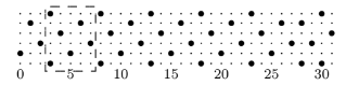
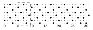
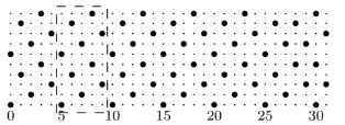
In Figures 2 to 4 we show the interior graphs used to construct dominating sets. In each we show a five column portion of the graph that can be repeated as necessary to get a cylinder with larger $n$ . We have omitted the edges in these graphs as the structure is apparent; the small dots are vertices, the large dots are vertices in the dominating sets.

Figure 2: Interior Subgraph $C_{32} P_{6}$

Figure 3: Interior Subgraph $C_{32} P_{8}$

Figure 4: Interior Subgraph $C_{32} P_{10}$

In Figures 5 to 8 we show the edge graphs used to construct dominating sets. Again, in each we show a five column portion of the graph that can be repeated as necessary to get a cylinder with larger $n$ .

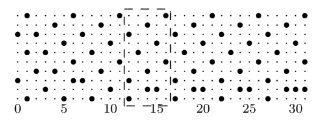
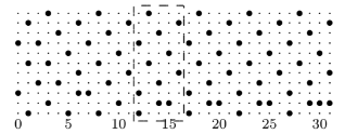
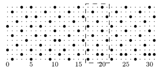
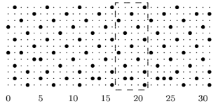
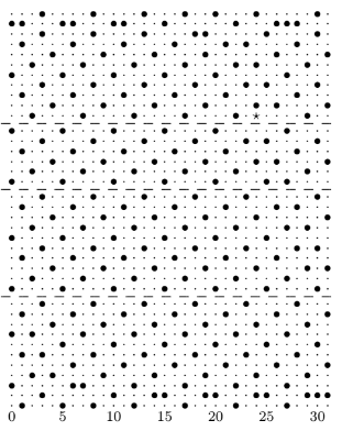
Finally, we show some examples of cylinders put together from these pieces. In the case of even $m$ , as mentioned above, we need an extra vertex in the dominating set; this vertex is shown as a star. The extra vertex is always in the bottom row of the top edge graph. Note also that to make the subgraphs fit together properly, so that we get a dominating set for the whole cylinder, some of the subgraphs must be rotated so that they line up properly at the boundaries, which are shown with dashed lines. (We produced in all twenty of these graphs, covering $23 \leq m \leq 42$ .)

Figure 9: Partitioned Cylinder $C_{32} P_{25}$ , $| S | = 174$

Figure 10: Partitioned Cylinder $C_{32} P_{26}$ , $| S | = 181$

Figure 11: Partitioned Cylinder $C_{32} P_{33}$ , $| S | = 226$

Figure 12: Partitioned Cylinder $C_{32} P_{34}$ , $| S | = 233$

Figure 13: Partitioned Cylinder $C_{32} P_{27}$ , $| S | = 252$

Figure 14: Partitioned Cylinder $C_{32} P_{38}$ , $| S | = 259$

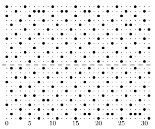
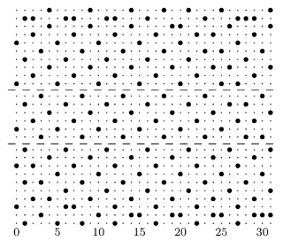
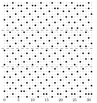
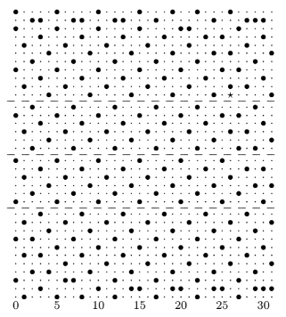
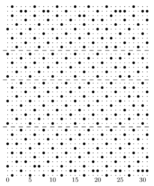
To produce a dominated cylinder of arbitrary size, we first determine which of the individual subgraphs we will need, namely, two edge subgraphs, some number of interior subgraphs with 10 rows, and one or two additional graphs with 6 or 8 rows. Then using the repeatable sections in the graphs of Figures 2 to 8, we expand each of these graphs to the desired number of columns, and finally we rotate the graphs as necessary so that they fit together properly.

We can now write down an upper bound for each $m$ and $n$ . For example, for $m \equiv 7 (\mod 10)$ and $m \geq 27$ , we use edge graphs with 11 and 10 rows, an interior graph with 6 rows, and as many additional interior subgraphs of 10 rows as needed. Let $m = 10 i + 7$ and $n = 5 k + 2$ . The number of vertices contributed by the edge graph with 11 rows is $77 + \frac{n - 32}{5} 12 = 12 k + 5$ , since the repeatable section, from Figure 6, contributes 12 vertices to the dominating set. Similarly, the edge graph with 10 vertices contributes $71 + \frac{n - 32}{5} 11 = 11 k + 5$ , an interior graph with 10 rows contributes $65 + (k - 6) 10 = 10 k + 5$ , and an interior graph with 6 rows contributes $39 + (k - 6) 6 = 6 k + 3$ . Then the total number of vertices in a dominating set is $\begin{aligned} (12 k + 5) + & (11 k + 5) + (6 k + 3) + (10 k + 5) \frac{m - 27}{10} \\ = (12 k + 5) + (11 k + 5) + (6 k + 3) + (10 k + 5) (i - 2) = 10 i k + 5 i + 9 k + 3, \end{aligned}$ which matches the corresponding lower bound in equation 3. We repeat this process for all other $j$ in $0, \dots, 9$ , with $m = 10 i + j$ , and in each case we find that the results match the values in equation 3. We also do $23 \leq m \leq 26$ as special cases, with no surprises.

5. Summary

For $m \geq 2$ and $n \geq 3$ , the domination number of $C_{n} P_{m}$ is now known when $n \equiv 0 (\mod 5)$ (as a result of P. Pavlič and J. Žerovnik [1] and José Juan Carreño et al. [2]) and $n \equiv 2 (\mod 5)$ . For the latter, when $m \geq 16$ or $m \geq n$ , the domination number is $⌈ \frac{\frac{4 n + 2}{10} m + \frac{4 n - 13}{5}}{2} ⌉,$ as shown here. For $m < 16$ and $n > m$ , the domination numbers are given by the formulas found in Crevals [6].

Unfortunately, the technique used here seems unlikely to settle the remaining cases, when $n$ is 1, 3, or $4 (\mod 5)$ . The lower bounds we get are below the upper bounds of [] by a small multiple of $m$ . When we look at a few sample subgraphs generated by our algorithm, they do not fit together nicely at the boundaries (that is, some vertices are left undominated), and so do not give upper bounds matching our lower bounds. Indeed, it seems quite remarkable that for $n \equiv 2 (\mod 5)$ the subgraphs can be combined to dominate the entire graph.

It is possible that our technique might work using somewhat larger subgraphs, though the algorithm we used would have to be improved or replaced with a substantially faster one. Computing the minimum wasted domination for fewer than 13 rows was reasonably fast on an Intel Core i7, although for 12 rows it did take a week or two. The 13 row graphs took considerably longer. We split the problem into 10 pieces by hand and ran each on a separate Intel Core i5 computer that was otherwise idle. The division wasn’t perfect, so some finished earlier than others; the whole process took over three months. The programs were written in C++ and compiled with the Gnu gcc compiler with optimization.

References:

Pavlic, P.O.L.O.N.A. and Zerovnik, J., 2013. A note on the domination number of the Cartesian products of paths and cycles. Kragujevac Journal of Mathematics, 37(2), pp.275-285.
Carreño, J.J., Martínez, J.A. and Puertas, M.L., 2020. A general lower bound for the domination number of cylindrical graphs. Bulletin of the Malaysian Mathematical Sciences Society, 43, pp.1671-1684.
Guichard, D.R., 2022. A New Lower Bound for the Domination Number of Complete Cylindrical Grid Graphs. arXiv preprint arXiv:2207.14414.
Livingston, M. and Stout, Q.F., 1994. Constant time computation of minimum dominating sets. Congressus Numerantium, pp.116-128.
Fisher, D.C., 1993. The domination number of complete grid graphs. preprint.
Crevals, S., 2014. Domination of cylinder graphs. Congressus Numerantium 219, pp.53-63.

[1] Pavlic, P.O.L.O.N.A. and Zerovnik, J., 2013. A note on the domination number of the Cartesian products of paths and cycles. Kragujevac Journal of Mathematics, 37(2), pp.275-285.

[2] Carreño, J.J., Martínez, J.A. and Puertas, M.L., 2020. A general lower bound for the domination number of cylindrical graphs. Bulletin of the Malaysian Mathematical Sciences Society, 43, pp.1671-1684.

[3] Guichard, D.R., 2022. A New Lower Bound for the Domination Number of Complete Cylindrical Grid Graphs. arXiv preprint arXiv:2207.14414.

[4] Livingston, M. and Stout, Q.F., 1994. Constant time computation of minimum dominating sets. Congressus Numerantium, pp.116-128.

[5] Fisher, D.C., 1993. The domination number of complete grid graphs. preprint.

[6] Crevals, S., 2014. Domination of cylinder graphs. Congressus Numerantium 219, pp.53-63.

Contents

Journal of Combinatorial Mathematics and Combinatorial Computing