
Graph theory is the study of graphs, a type of mathematical structure used to depict interactions between two entities. Graphs are one of the most ubiquitous data structures, used in fields as diverse as physics, sociology, architecture, chemistry, genetics, electrical engineering, operational research, and linguistics to model a wide range of linkages and processes. In this paper, we study graph resolvability, an essential concept in metric graph theory that is used in facility placement problems, networking, robot navigation, mathematical and pharmaceutical chemistry, and Mastermind games.
Over 3000 problems have been identified as NP-complete. Many practical issues, such as routing, fault tolerance, coding, embedding, resolvability, and coloring, lend themselves naturally to modeling and explanation using graph theoretical language [1]. Studies of the metric properties of graphs, such as the metric dimension and fault-tolerant metric dimension, have become increasingly popular over the past few decades due to their practical applications.
In 1975, Slater (and, independently, Harary and Melter) introduced the concept of the metric dimension. Recent progress has been made with the introduction of the fault-tolerant metric dimension [2,3]. Censors are defined as metric base components in [4]. If some censors fail, we may not have enough data to handle the threat (e.g., fire, intruder). Hernando et al. developed the concept of the fault-tolerant metric dimension to address such issues [5]. A fault-tolerant resolving set continues to provide accurate results even if one of the censors fails. Consequently, the fault-tolerant metric dimension is useful in all scenarios where the traditional metric dimension has found applications.
Raza et al. investigated the fault-tolerant metric dimension of some families of convex polytopes [6]. Fault-tolerant resolvability in specific crystal structures was explored in [7]. Sharma and Bhat studied the fault-tolerant metric dimensions of a two-fold heptagonal-nonagonal circular ladder [8]. They demonstrated that such a ladder has the same metric dimension as a ladder with the same number of rungs. Additionally, they explored its fault-tolerant metric dimension, showing that the metric basis and the edge metric basis are distinct. For more information on fault-tolerant metric dimensions, we encourage interested readers to consult the literature [9-12]. In this paper, we only analyze basic graphs that are connected and undirected.
A graph, denoted by the letter \(G\), consists of two sets: the vertex set, denoted \(V(G)\), and the edge set, denoted \(E(G)\). The components of \(V(G)\) and \(E(G)\), known as the vertices and edges of \(G\), respectively, form the graph \(G\). In a graph, the length of the path connecting two vertices is called the distance between those vertices. The distances between two vertices \(p\) and \(q\) with respect to the set \(R\) are represented by \(d(p|R)\) and \(d(q|R)\), respectively. A vertex set \(R \subseteq V(G)\) is said to resolve the underlying graph \(G\) if, for any two vertices \(p, q \in V(G)\), there exists a vertex \(x \in R\) that resolves \(p\) and \(q\). Two vertices \(x, y \in G\) are resolved by a vertex \(s \in G\) if \(d(x|s) \neq d(y|s)\). There may be multiple resolving sets for a graph. The set \(V(G)\) is trivially a resolving set. The minimum cardinality of a resolving set in \(G\) is called its metric dimension, denoted by \(\beta(G)\) [13].
A resolving set \(R\) is fault-tolerant if, for every \(p \in R\), \(R – p\) preserves the property of being a resolving set. Analogous to the metric dimension, the fault-tolerant metric dimension is the minimum number \(\beta'(G)\) such that there exists a fault-tolerant resolving set of order \(\beta'(G)\). A fault-tolerant resolving set of minimal order is called the fault-tolerant metric dimension of \(G\) [13]. The objective of this study is to classify arithmetic graphs according to their fault-tolerant metric dimension. Arithmetic graphs are important in applications such as aircraft design, electronic circuit design, computer engineering, and transportation systems because of their ability to model complex networks.
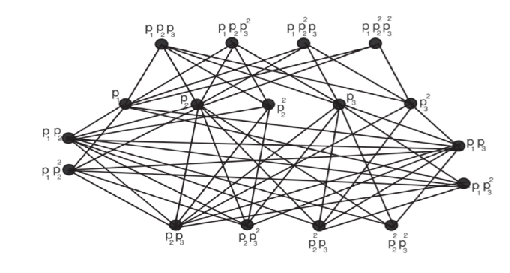
The arithmetic graph \(A_l\) is defined as the graph whose vertex set is the set of all divisors of a composite number \(l\), where \(l = p_1^{\gamma_1} p_2^{\eta_2} \cdots p_n^{\alpha_n}\), and \(p_i\)’s are distinct primes with \(p_i \geq 2\). Two distinct divisors \(x\) and \(y\) of \(l\) are said to have the same parity if they have the same prime factors (e.g., \(x = p_1 p_2\) and \(y = p_1^2 p_2^3\) have the same parity). Furthermore, two distinct vertices \(x, y \in A_l\) are adjacent if and only if they have different parity and \(\gcd(x, y) = p_i\) (greatest common divisor) for some \(i \in \{1, 2, \dots, t\}\) (see Figure 1) [14].
The main results of this paper are discussed in this section.
Theorem 1. Let \(A_l\) be an arithmetic graph, where \(l\) is a composite number with the canonical form \(l = p_1^\gamma p_2^\eta\), and \(\gamma, \eta \geq 1\). Then:
\(\beta'(A_l) = 2\), for \(\gamma = 1\), \(\eta = 1\).
\(\beta'(A_l) = 2\eta\), for \(\gamma = 1\), \(\eta > 1\).
\(\beta'(A_l) = 6\), for \(\gamma = 2\), \(\eta = 2\).
\(\beta'(A_l) = (\gamma + 1)(\eta + 1) – 2\), for \(\gamma, \eta > 2\).
Proof. The set of vertices for the arithmetic graph \(A_l\) is
\[V_l = \{ p^{\gamma}_1, p^{\eta}_2, p^{\gamma}_1 p_2, p_1 p^{\eta}_2, p^{\gamma}_1 p^{\gamma}_2 \}\] where \(1 \leq \gamma, \eta \leq n\). We will differentiate the proof into four cases.
Case 1. For \(\gamma = 1\) and \(\eta = 1\), we have
\[V_l = \{ p_1, p_2, p_1 p_2 \}.\]
Consider the set \(R = \{ p_1, p_2 \} \subseteq V_l\). The distances are calculated as follows:
\[d(p_1 \mid R) = (0, 2), \quad d(p_2 \mid R) = (2, 0), \quad d(p_1 p_2 \mid R) = (1, 1).\]
Since all the distances are distinct, \(R\) is a resolving set.
Next, we will prove that \(R – \{v\} = R'\) is also a resolving set, where \(v\) is any vertex that is a member of \(R\). Let \(p_2 \in R\). Then,
\[R – \{p_2\} = \{p_1\} = R'.\]
Now, the distances are:
\[d\left(p_1 \mid R'\right) = (0), \quad d(p_2 \mid R') = 2, \quad d(p_1 p_2 \mid R') = 1.\]
Since all the distances are distinct, \(R'\) is also a resolving set. Therefore, \(R\) is a fault-tolerant resolving set with
\[\beta'(A_l) = 2.\]
Case 2. For \(\gamma = 1\) and \(\eta \geq 2\), the set of vertices is
\[V_l = \{ p_1, p_2, p^2_2, \ldots, p^{\eta}_2, p_1 p_2, p_1 p^2_2, \ldots, p^{\gamma}_1 p^{\eta}_2 \}.\]
Consider the set
\[R = \{ p_1, p_2, p^2_2, \ldots, p^{\eta}_2, p_1 p^2_2, \ldots, p^{\gamma}_1 p^{\eta}_2 \} \subseteq V_l.\]
Now, we calculate the distances:
\[\begin{aligned} d(p_1 \mid R) &= (0, 2, 2, \ldots, 2, 1, \ldots, 1),\\ d(p_2 \mid R) &= (2, 0, 2, \ldots, 2, 1, \ldots, 1),\\ d(p^2_2 \mid R)& = (2, 2, 0, 2, \ldots, 2, 3, \ldots, 3),\\ d(p^{\eta}_2 \mid R)& = (2, 2, 2, \ldots, 2, 0, 3, 3, \ldots, 3),\\ d(p_1 p_2 \mid R)& = (1, 1, \ldots, 1, 2, \ldots, 2),\\ d(p_1 p^2_2 \mid R) &= (1, 1, 3, \ldots, 3, 0, 2, \ldots, 2),\\ d(p_1 p^{\eta-1}_2 \mid R) &= (1, 3, \ldots, 3, 2, \ldots, 2, 0, 2),\\ d(p_1 p^{\eta}_2 \mid R)& = (1, 1, 3, \ldots, 3, 2, \ldots, 2, 0). \end{aligned}\]
Since all the distances are distinct, \(R\) is a resolving set. Now we will prove that \(R – \{v\} = R'\) is also a resolving set, where \(v\) is any vertex that is a member of \(R\). Let \(p_1 \in R\). Then,
\[R – \{p_1\} = R' = \{ p_2, p^2_2, \ldots, p^{\eta}_2, p_1 p^2_2, \ldots, p_1 p^{\eta}_2 \}.\]
Now, we calculate the distances:
\[\begin{aligned} d(p_1 \mid R')& = (2, 2, \ldots, 2, 1, \ldots, 1),\\ d(p_2 \mid R') &= (0, 2, \ldots, 2, 1, \ldots, 1),\\ d(p^2_2 \mid R') &= (2, 0, 2, \ldots, 2, 3, \ldots, 3),\\ d(p_1 p_2 \mid R')& = (1, \ldots, 1, 2, \ldots, 2),\\ d(p_1 p^2_2 \mid R') &= (1, 3, \ldots, 3, 0, 2, \ldots, 2),\\ d(p_1 p^{\eta-1}_2 \mid R') &= (1, 3, \ldots, 3, 2, \ldots, 2, 0, 2),\\ d(p_1 p^{\eta}_2 \mid R')& = (1, 3, \ldots, 3, 2, \ldots, 2, 0). \end{aligned}\]
Since all the distances are distinct, \(R'\) is also a resolving set. Therefore, the fault-tolerant metric dimension of \(A_l\) is \(2\eta\).
Next, we will prove the minimality of the fault-tolerant resolving set \(R\). Consider the set \(R' – \{v\} = R''\), where \(v\) is any vertex that is a member of \(R'\). Let \(p_2 \in R'\). Then,
\[R' – \{p_2\} = R'' = \{ p^2_2, \ldots, p^{\eta}_2, p_1 p^2_2, \ldots, p^{\gamma}_1 p^{\eta}_2 \}.\]
Now, we calculate the distances:
\[\begin{aligned} d(p_1 \mid R'')& = (2, 2, \ldots, 2, 1, \ldots, 1),\\ d(p_2 \mid R'') &= (2, 2, \ldots, 2, 1, \ldots, 1). \end{aligned}\]
Since the distances are the same, the set \(R\) is a minimal fault-tolerant resolving set. Hence, the minimum cardinality of the fault-tolerant resolving set is \(2\eta\).
Case 3. For \(\gamma, \ \eta = 2, \ V_l = \{p_1, \ p_2, \ p^2_1, \ p^2_2, \ p_1 p_2, \ p_1 p^2_2, \ p^2_1 p_2, \ p^2_1 p^2_2\}\). Consider the resolving set
\[\begin{aligned} R = \{p_1, \ p_2, \ p^2_1, \ p^2_2, \ p_1 p^2_2, \ p^2_1 p_2\} \subseteq V_l. \end{aligned}\]
Now, we compute the distances:
\[\begin{aligned} d(p_1 | R) & = (0, 2, 2, 2, 1, 1), \\ d(p_2 | R) & = (2, 0, 2, 2, 1, 1), \\ d(p^2_1 | R) & = (2, 2, 0, 2, 1, 3), \\ d(p^2_2 | R) & = (2, 2, 2, 0, 3, 1), \\ d(p_1 p_2 | R) & = (1, 1, 1, 1, 2, 2), \\ d(p^2_1 p_2 | R) & = (1, 1, 3, 1, 2, 0), \\ d(p_1 p^2_2 | R) & = (1, 1, 1, 3, 0, 2), \\ d(p^2_1 p^2_2 | R) & = (1, 1, 3, 3, 2, 2). \end{aligned}\]
Since all the distances are distinct, \(R\) is a resolving set. Now we will prove that \(R – \{v\} = R'\) is also a resolving set, where \(v\) is any vertex that is a member of \(R\). Let \(p_1 \in R\). Then, \(R – \{p_1\} = R'\).
\[\begin{aligned} R' &= \{p_2, \ p^2_1, \ p^2_2, \ p_1 p^2_2, \ p^2_1 p_2\}. \end{aligned}\]\[\begin{aligned} d(p_1 | R') & = (2, 2, 2, 1, 1), \\ d(p_2 | R') & = (0, 2, 2, 1, 1), \\ d(p^2_1 | R') & = (2, 0, 2, 1, 3), \\ d(p^2_2 | R') & = (2, 2, 0, 3, 1), \\ d(p_1 p_2 | R') & = (1, 1, 1, 2, 2), \\ d(p^2_1 p_2 | R') & = (1, 3, 1, 2, 0), \\ d(p_1 p^2_2 | R') & = (1, 1, 3, 0, 2), \\ d(p^2_1 p^2_2 | R') & = (1, 3, 3, 2, 2). \end{aligned}\]
Since all the distances are distinct, \(R'\) is also a resolving set. Thus, the fault-tolerant metric dimension of \(A_l = 6\).
Now we will prove the minimality of the fault-tolerant resolving set \(R\). Consider the set \(R' – \{v\} = R''\), where \(v\) is any vertex that is a member of \(R'\). Let \(p_2 \in R'\). Then, \(R' – \{p_2\} = R'' = \{p^2_1, \ p^2_2, \ p_1 p^2_2, \ p^2_1 p_2\}\).
Now, we compute the distances:
\[\begin{aligned} d(p_1 | R'') & = (2, 2, 1, 1), \\ d(p_2 | R'') & = (2, 2, 1, 1). \end{aligned}\]
Since the distances are the same, the set \(R\) is a minimal fault-tolerant resolving set. Hence, the minimum cardinality of the fault-tolerant resolving set is \(6\).
Case 4. For \(\gamma, \eta \geq 2\), let
\[V_l = \left\{ p_1, p_2, p_1^2, \ldots, p_1^\gamma, p_2^2, \ldots, p_2^\eta, p_1 p_2, p_1^2 p_2, \ldots, p_1^\gamma p_2 \right\},\] \[\left\{ p_1 p_2^2, \ldots, p_1 p_2^\eta, p_1^2 p_2^2, \ldots, p_1^\gamma p_2^\eta \right\}.\]
Consider the set
\[R = \{ p_1, p_2, p_1^2, \ldots, p_1^\gamma, p_2^2, \ldots, p_2^\eta, p_1^2 p_2, \ldots, p_1^\gamma p_2, p_1 p_2^2, \ldots, p_1 p_2^\eta, p_1^2 p_2^2, \ldots, p_1^\gamma p_2^\eta \} \subseteq V_l.\]
Now, we compute the distances:
\[\begin{aligned} d(p_1 | R) &= (0, 2, 2, \ldots, 2, 2, \ldots, 2, 1, \ldots, 1, 1, \ldots, 1, 1, \ldots, 1, 1), \\ d(p_2 | R) &= (2, 0, 2, \ldots, 2, 2, \ldots, 2, 1, \ldots, 1, 1, \ldots, 1, 1, \ldots, 1), \\ d(p_1^2 | R) &= (2, 2, 0, 2, \ldots, 2, 3, \ldots, 3, 1, \ldots, 1, 3, \ldots, 3, 3, \ldots, 3), \\ \vdots \\ d(p_1^\gamma | R) &= (2, 2, 2, \ldots, 2, 0, 3, \ldots, 3, 1, \ldots, 1, 3, \ldots, 3, 3, \ldots, 3), \\ d(p_2^2 | R) &= (2, 2, 2, \ldots, 2, 0, 2, \ldots, 2, 1, \ldots, 1, 3, \ldots, 3, 3, \ldots, 3), \\ d(p_2^3 | R) &= (2, 2, 2, \ldots, 2, 2, 0, 2, \ldots, 2), \\ \vdots \\ d(p_2^\eta | R) &= (2, 2, 2, \ldots, 2, 2, \ldots, 2, 0, 1, \ldots, 1, 3, \ldots, 3, 3, \ldots, 3), \\ d(p_1 p_2 | R) &= (1, 1, \ldots, 1, 1, \ldots, 1, 2, \ldots, 2, 2, \ldots, 2, 2, \ldots, 2), \\ d(p_1^2 p_2 | R) &= (1, 1, 3, \ldots, 3, 1, \ldots, 1, 0, 2, \ldots, 2, 2, \ldots, 2, 2, \ldots, 2), \\ \vdots \\ d(p_1^\gamma p_2 | R) &= (1, 1, 3, \ldots, 3, 1, \ldots, 1, 2, \ldots, 2, 0, 2, \ldots, 2, 2, \ldots, 2), \\ d(p_1 p_2^2 | R) &= (1, 1, 1, \ldots, 1, 3, \ldots, 3, 2, \ldots, 2, 0, 2, \ldots, 2, 2, \ldots, 2), \\ d(p_1 p_2^3 | R) &= (1, 1, 1, \ldots, 1, 3, \ldots, 3, 2, \ldots, 2, 2, 0, 2, \ldots, 2, 2, \ldots, 2), \\ \vdots \\ d(p_1 p_2^\eta | R) &= (1, 1, 1, \ldots, 1, 3, \ldots, 3, 2, \ldots, 2, 2, 2, \ldots, 2, 0, 2, \ldots, 2), \\ d(p_1^2 p_2^2 | R) &= (1, 1, 3, \ldots, 3, 3, \ldots, 3, 2, \ldots, 2, 2, \ldots, 2, 0, 2, \ldots, 2), \\ d(p_1^2 p_2^3 | R) &= (1, 1, 3, \ldots, 3, 3, \ldots, 3, 2, \ldots, 2, 2, \ldots, 2, 2, 0, 2, \ldots, 2), \\ \vdots \\ d(p_1^\gamma p_2^\eta | R) &= (1, 1, 3, \ldots, 3, 3, \ldots, 3, 2, \ldots, 2, 2, \ldots, 2, 2, \ldots, 2, 0). \end{aligned}\]
Since all distances are distinct, \(R'\) is a resolving set. This concludes the proof for this case. ◻
Theorem 2. Let \(l\) be a composite number expressed in its canonical form as \(l = p_1^{\gamma} p_2^{\eta} p_3^{\xi}\), where \(\gamma, \eta, \xi \geq 1\). Then the following holds:
\(\beta'(A_l) = 4\) for \(\gamma = 1, \eta = 1, \xi = 1\).
\(\beta'(A_l) = 6\) for \(\gamma = 2, \eta = 1, \xi = 1\).
\(\beta'(A_l) = 4(\gamma – 1)\) for \(\gamma > 2, \eta = 1, \xi = 1\).
\(\beta'(A_l) = 9\) for \(\gamma = 2, \eta = 2, \xi = 1\).
\(\beta'(A_l) = 2(\gamma + 1)(\eta + 1) – 8\) for \(\gamma > 2, \eta > 2, \xi = 1\).
\(\beta'(A_l) = 15\) for \(\gamma = 2, \eta = 2, \xi = 2\).
\(\beta'(A_l) = (\gamma + 1)(\eta + 1)(\xi + 1) – 8\) for \(\gamma > 2, \eta > 2, \xi > 2\).
Proof. The set of vertices for the arithmetic graph \(A_l\) is given by
\[\begin{aligned} V_l =& \left\{p_1^{\gamma}, p_2^{\eta}, p_3^{\xi}, p_1^{\gamma} p_2, p_1^{\gamma} p_3, p_1 p_2^{\eta}, p_2 p_3^{\xi}, p_1 p_3^{\xi}, p_1^{\gamma} p_2^{\eta}, p_1^{\gamma} p_3^{\xi}, p_2^{\eta} p_3^{\xi}, p_1^{\gamma} p_2 p_3, p_1 p_2^{\eta} p_3, p_1 p_2 p_3^{\xi}, p_1^{\gamma} p_2^{\eta} p_3,\right.\\ &\left.p_1^{\gamma} p_2 p_3^{\xi}, p_1 p_2^{\eta} p_3^{\xi}, p_1^{\gamma} p_2^{\eta} p_3^{\xi}\right\} \end{aligned}\]
where \(1 \leq \gamma, \eta, \xi \leq n\). We will proceed with the proof by considering seven distinct cases.
Case 1. For \(\gamma = 1, \eta = 1, \xi = 1\), we have
\[V_l = \{p_1, p_2, p_3, p_1 p_2, p_1 p_3, p_2 p_3, p_1 p_2 p_3\}.\]
Let us consider the subset
\[R = \{p_1 p_2, p_1 p_3, p_2 p_3, p_1 p_2 p_3\} \subseteq V_l.\]
The distances from the vertices to the set \(R\) are calculated as follows:
\[\begin{aligned} d\left(p_1 \middle| R\right) & = (1, 1, 2, 1), \\ d\left(p_2 \middle| R\right) & = (1, 2, 1, 1), \\ d\left(p_3 \middle| R\right) & = (2, 1, 1, 1), \\ d\left(p_1 p_2 \middle| R\right) & = (0, 1, 1, 2), \\ d\left(p_1 p_3 \middle| R\right) & = (1, 0, 1, 2), \\ d\left(p_2 p_3 \middle| R\right) & = (1, 1, 0, 2), \\ d\left(p_1 p_2 p_3 \middle| R\right) & = (2, 2, 2, 0). \end{aligned}\]
Since all the distances are distinct, the set \(R\) is a resolving set. Now, we will show that the set \(R' = R \setminus \{v\}\) is also a resolving set, where \(v\) is any vertex in \(R\).
Assume \(p_1 p_2 \in R\). Then,
\[R' = \{p_1 p_3, p_2 p_3, p_1 p_2 p_3\}.\]
Calculating the distances for the vertices with respect to \(R'\): \[\begin{aligned} d\left(p_1 \middle| R'\right) & = (1, 2, 1), \\ d\left(p_2 \middle| R'\right) & = (2, 1, 1), \\ d\left(p_3 \middle| R'\right) & = (1, 1, 1), \\ d\left(p_1 p_2 \middle| R'\right) & = (1, 1, 2), \\ d\left(p_1 p_3 \middle| R'\right) & = (0, 1, 2), \\ d\left(p_2 p_3 \middle| R'\right) & = (1, 0, 2), \\ d\left(p_1 p_2 p_3 \middle| R'\right) & = (2, 2, 0). \end{aligned}\]
Since all the distances are distinct, \(R'\) is also a resolving set.
Next, we will establish the minimality of the fault-tolerant resolving set \(R\). Consider the set \(R'' = R' \setminus \{v\}\), where \(v\) is any vertex in \(R'\). Let \(p_1 p_3 \in R'\). Then,
\[R'' = \{p_2 p_3, p_1 p_2 p_3\}.\]
Calculating the distances gives us:
\[\begin{aligned} d\left(p_1 p_2 \middle| R''\right) & = (1, 2), \\ d\left(p_1 p_3 \middle| R''\right) & = (1, 2). \end{aligned}\]
Since the distances are not distinct, \(R''\) is not a resolving set. Therefore, the minimum cardinality of the fault-tolerant resolving set is \(4\).
Case 2. For \(\gamma = 2, \ \eta, \ \xi = 1\),
\[V_l = \{ p_1, p_2, p_3, p_1^2, p_1 p_2, p_1^2 p_2, p_1 p_3, p_1^2 p_3, p_2 p_3, p_1 p_2 p_3, p_1^2 p_2 p_3 \}\]
Let the set \(R = \{ p_1^2 p_2, p_1 p_3, p_1^2 p_3, p_2 p_3, p_1 p_2 p_3, p_1^2 p_2 p_3 \} \subseteq V_l\).
Now, we calculate the distances: \[\begin{aligned} d(p_1 | R) & = (1, 1, 1, 2, 1, 1), \\ d(p_2 | R) & = (1, 2, 2, 1, 1, 1), \\ d(p_3 | R) & = (2, 1, 1, 1, 1, 1), \\ d(p_1^2 | R) & = (2, 1, 2, 2, 1, 3), \\ d(p_1 p_2 | R) & = (2, 1, 1, 1, 2, 2), \\ d(p_1^2 p_2 | R) & = (0, 1, 2, 2, 2, 2), \\ d(p_1 p_3 | R) & = (1, 0, 2, 1, 2, 2), \\ d(p_1^2 p_3 | R) & = (2, 2, 0, 1, 2, 2), \\ d(p_2 p_3 | R) & = (1, 1, 1, 0, 2, 2), \\ d(p_1 p_2 p_3 | R) & = (2, 2, 2, 2, 0, 2), \\ d(p_1^2 p_2 p_3 | R) & = (2, 2, 2, 2, 2, 0). \end{aligned}\] Since all the distances are distinct, \(R\) is a resolving set.
Next, we will prove that \(R' = R – \{v\}\) is also a resolving set, where \(v\) is any vertex in \(R\). Let \(p_1 p_2 p_3 \in R\). Then, \(R' = R – \{p_1 p_2 p_3\}\).
Now, \(R' = \{ p_1^2 p_2, p_1 p_3, p_1^2 p_3, p_2 p_3, p_1^2 p_2 p_3 \}\). The distances with respect to \(R'\) are: \[\begin{aligned} d(p_1 | R') & = (1, 1, 1, 2, 1), \\ d(p_2 | R') & = (1, 2, 2, 1, 1), \\ d(p_3 | R') & = (2, 1, 1, 1, 1), \\ d(p_1^2 | R') & = (2, 1, 2, 2, 3), \\ d(p_1 p_2 | R') & = (2, 1, 1, 1, 2), \\ d(p_1^2 p_2 | R') & = (0, 1, 2, 2, 2), \\ d(p_1 p_3 | R') & = (1, 0, 2, 1, 2), \\ d(p_1^2 p_3 | R') & = (2, 2, 0, 1, 2), \\ d(p_2 p_3 | R') & = (1, 1, 1, 0, 2), \\ d(p_1 p_2 p_3 | R') & = (2, 2, 2, 2, 2), \\ d(p_1^2 p_2 p_3 | R') & = (2, 2, 2, 2, 0). \end{aligned}\] Since all the distances are distinct, \(R'\) is also a resolving set.
Finally, we will prove the minimality of the fault-tolerant resolving set \(R\). Consider the set \(R'' = R' – \{v\}\), where \(v\) is any vertex in \(R'\). Let \(p_1^2 p_2 p_3 \in R'\). Then, \(R'' = R' – \{p_1^2, p_2 p_3\}\).
Now, \(R'' = \{ p_1^2 p_2, p_1 p_3, p_1^2 p_3, p_2 p_3 \}\). The distances with respect to \(R''\) are:
\[d(p_1 p_2 p_3 | R'') = (2, 2, 2, 2), \quad d(p_1^2 p_2 p_3 | R'') = (2, 2, 2, 2).\]
Since the distances are not distinct, \(R''\) is not a resolving set. Thus, the minimum cardinality of the fault-tolerant resolving set is \(6\).
Case 3. For \(\gamma > 2,\ \eta,\ \xi = 1\), the set \(V_l\) is defined as: \[\begin{aligned} V_l =& \left\{ p_1, p_2, p_3, p_1^2, \ldots, p_1^\gamma, p_1 p_2, p_1^2 p_2, \ldots, p_1^\gamma p_2, p_1 p_3, p_1^2 p_3,\right. \\ &\left.\ldots, p_1^\gamma p_3, p_2 p_3, p_1 p_2 p_3, p_1^2 p_2 p_3, \ldots, p_1^\gamma p_2 p_3 \right\}. \end{aligned}\] Let the set \[R = \{ p_1^2, \ldots, p_1^\gamma, p_1^2 p_2, \ldots, p_1^\gamma p_2, p_1^2 p_3, \ldots, p_1^\gamma p_3, p_1^2 p_2 p_3, \ldots, p_1^\gamma p_2 p_3 \} \subseteq V_l\] be the resolving set.
Now we compute the distances: \[\begin{aligned} d(p_1 | R) &= (2, \ldots, 2, 1, \ldots, 1, 1, \ldots, 1, 1, \ldots, 1), \\ d(p_2 | R) &= (2, \ldots, 2, 1, \ldots, 1, 2, \ldots, 2, 1, \ldots, 1), \\ d(p_3 | R) &= (2, \ldots, 2, 2, \ldots, 2, 1, \ldots, 1, 1, \ldots, 1), \\ d(p_1^2 | R) &= (0, 2, \ldots, 2, 2, \ldots, 2, 2, \ldots, 2, 2, 3, \ldots, 3), \\ d(p_1^3 | R) &= (2, 0, 2, \ldots, 2, 2, \ldots, 2, 2, \ldots, 2, 2, 3, \ldots, 3), \\ &\vdots \\ d(p_1^\gamma | R) &= (2, \ldots, 2, 0, 2, \ldots, 2, 2, \ldots, 2, 2, 3, \ldots, 3), \\ d(p_1 p_2 | R) &= (1, \ldots, 1, 2, \ldots, 2, 1, \ldots, 1, 2, \ldots, 2), \\ d(p_1^2 p_2 | R) &= (2, \ldots, 2, 0, 2, \ldots, 2, 2, \ldots, 2, 2, \ldots, 2), \\ d(p_1^3 p_2 | R) &= (2, \ldots, 2, 2, 0, 2, \ldots, 2, 2, \ldots, 2), \\ &\vdots \\ d(p_1^\gamma p_2 | R) &= (2, \ldots, 2, 2, \ldots, 2, 0, 2, \ldots, 2), \\ d(p_1 p_3 | R) &= (1, \ldots, 1, 1, \ldots, 1, 2, \ldots, 2, 2, \ldots, 2), \\ d(p_1^2 p_3 | R) &= (2, \ldots, 2, 2, \ldots, 2, 0, 2, \ldots, 2), \\ d(p_1^3 p_3 | R) &= (2, \ldots, 2, 2, \ldots, 2, 0, 2, \ldots, 2), \\ &\vdots \\ d(p_1^\gamma p_3 | R) &= (2, \ldots, 2, 2, \ldots, 2, 2, \ldots, 2, 0, 2, \ldots, 2), \\ d(p_2 p_3 | R) &= (2, \ldots, 2, 1, \ldots, 1, 2, \ldots, 2, 2, \ldots, 2), \\ d(p_1 p_2 p_3 | R) &= (1, \ldots, 1, 2, \ldots, 2, 2, \ldots, 2, 2, \ldots, 2), \\ d(p_1^2 p_2 p_3 | R) &= (3, \ldots, 3, 2, \ldots, 2, 2, 2, 0, 2, \ldots, 2), \\ &\vdots \\ d(p_1^\gamma p_2^\eta p_3^\xi | R) &= (3, \ldots, 3, 2, \ldots, 2, 2, \ldots, 2, 2, \ldots, 2, 0). \end{aligned}\]
Since all distances are unique, \(R\) is a resolving set.
Now, we will prove that \(R – \{v\} = R'\) is also a resolving set, where \(v\) is any vertex that is a member of \(R\). Let \(p_1^2 \in R\). Then, \(R – \{p_1^2\} = R'\).
\[R' = \{ p_1^3, \ldots, p_1^\gamma, p_1^2 p_2, \ldots, p_1^\gamma p_2, p_1^2 p_3, \ldots, p_1^\gamma p_3, p_1^2 p_2 p_3, \ldots, p_1^\gamma p_2 p_3 \}.\]
Now we compute the distances in \(R'\): \[\begin{aligned} d(p_1 | R') &= (2, \ldots, 2, 1, \ldots, 1, 1, \ldots, 1, 1, \ldots, 1), \\ d(p_2 | R') &= (2, \ldots, 2, 1, \ldots, 1, 2, \ldots, 2, 1, \ldots, 1), \\ d(p_3 | R') &= (2, \ldots, 2, 2, \ldots, 2, 1, \ldots, 1, 1, \ldots, 1), \\ d(p_1^2 | R') &= (2, \ldots, 2, 2, \ldots, 2, 2, \ldots, 2, 2, 3, \ldots, 3), \\ d(p_1^3 | R') &= (0, 2, \ldots, 2, 2, \ldots, 2, 2, \ldots, 2, 2, 3, \ldots, 3), \\ &\vdots \\ d(p_1^\gamma | R') &= (2, \ldots, 2, 0, 2, \ldots, 2, 2, \ldots, 2, 2, 3, \ldots, 3), \\ d(p_1 p_2 | R') &= (1, \ldots, 1, 2, \ldots, 2, 1, \ldots, 1, 2, \ldots, 2), \\ d(p_1^2 p_2 | R') &= (2, \ldots, 2, 0, 2, \ldots, 2, 2, \ldots, 2, 2, \ldots, 2), \\ d(p_1^3 p_2 | R') &= (2, \ldots, 2, 2, 0, 2, \ldots, 2, 2, \ldots, 2), \\ &\vdots \\ d(p_1^\gamma p_2 | R') &= (2, \ldots, 2, 2, \ldots, 2, 0, 2, \ldots, 2), \\ d(p_1 p_3 | R') &= (1, \ldots, 1, 1, \ldots, 1, 2, \ldots, 2, 2, \ldots, 2), \\ d(p_1^2 p_3 | R') &= (2, \ldots, 2, 2, \ldots, 2, 0, 2, \ldots, 2), \\ d(p_1^3 p_3 | R') &= (2, \ldots, 2, 2, \ldots, 2, 0, 2, \ldots, 2), \\ &\vdots \\ d(p_1^\gamma p_3 | R') &= (2, \ldots, 2, 2, \ldots, 2, 2, \ldots, 2, 0, 2, \ldots, 2), \\ d(p_2 p_3 | R') &= (2, \ldots, 2, 1, \ldots, 1, 2, \ldots, 2, 2, \ldots, 2), \\ d(p_1 p_2 p_3 | R') &= (1, \ldots, 1, 2, \ldots, 2, 2, \ldots, 2, 2, \ldots, 2), \\ d(p_1^2 p_2 p_3 | R') &= (3, \ldots, 3, 2, \ldots, 2, 2, 2, 0, 2, \ldots, 2), \\ &\vdots \\ d(p_1^\gamma p_2^\eta p_3^\xi | R') &= (3, \ldots, 3, 2, \ldots, 2, 2, \ldots, 2, 2, \ldots, 2, 0). \end{aligned}\]
Thus, since \(R'\) generates unique distances, it is also a resolving set.
Case 4. For \(\gamma, \eta = 2, \xi = 1\).
Let \[\begin{aligned} V_l =& \left\{p_1, p_2, p_3, p_1^2, p_2^2, p_1 p_2, p_1^2 p_2, p_1 p_3, p_1^2 p_3, p_1^2 p_2^2, p_1 p_2^2, p_2 p_3,\right.\\ &\left. p_2^2 p_3, p_1 p_2 p_3, p_1^2 p_2 p_3, p_1 p_2^2 p_3, p_1^2 p_2^2 p_3\right\}. \end{aligned}\]
Let the set
\[R = \{p_1^2 p_2, p_1^2 p_3, p_1^2 p_2^2, p_1 p_2^2, p_2^2 p_3, p_1 p_2 p_3, p_1^2 p_2 p_3, p_1 p_2^2 p_3, p_1^2 p_2^2 p_3\} \subseteq V_l.\]
Now, we compute the distances: \[\begin{aligned} d(p_1 | R) & = (1, 1, 1, 1, 2, 1, 1, 1, 1), \\ d(p_2 | R) & = (1, 2, 1, 1, 1, 1, 1, 1, 1), \\ d(p_3 | R) & = (2, 1, 2, 2, 1, 1, 1, 1, 1), \\ d(p_1^2 | R) & = (1, 1, 2, 2, 2, 1, 3, 1, 3), \\ d(p_2^2 | R) & = (1, 2, 2, 2, 2, 1, 1, 3, 3), \\ d(p_1 p_2 | R) & = (2, 1, 2, 2, 1, 2, 2, 2, 2), \\ d(p_1^2 p_2 | R) & = (0, 2, 2, 2, 1, 2, 2, 2, 2), \\ d(p_1 p_3 | R) & = (1, 2, 1, 1, 1, 2, 2, 2, 2), \\ d(p_1^2 p_3 | R) & = (2, 0, 2, 1, 1, 2, 2, 2, 2), \\ d(p_1^2 p_2^2 | R) & = (2, 2, 0, 2, 2, 2, 2, 2, 2), \\ d(p_1 p_2^2 | R) & = (2, 1, 2, 0, 2, 2, 2, 2, 2), \\ d(p_2 p_3 | R) & = (1, 1, 1, 1, 2, 2, 2, 2, 2), \\ d(p_2^2 p_3 | R) & = (1, 1, 2, 2, 0, 2, 2, 2, 2), \\ d(p_1 p_2 p_3 | R) & = (2, 2, 2, 2, 0, 2, 2, 2, 2), \\ d(p_1^2 p_2 p_3 | R) & = (2, 2, 2, 2, 2, 2, 0, 2, 2). \end{aligned}\] Since all the distances are distinct, \(R\) is a resolving set.
Now, we will prove that \(R – \{v\} = R'\) is also a resolving set, where \(v\) is any vertex that is a member of \(R\).
Let \(p_1 p_2 p_3 \in R\). Then \(R – \{p_1 p_2 p_3\} = R'\) such that
\[R' = \{p_1^2 p_2, p_1^2 p_3, p_1^2 p_2^2, p_1 p_2^2, p_2^2 p_3, p_1 p_2 p_3, p_1^2 p_2 p_3, p_1 p_2^2 p_3, p_1^2 p_2^2 p_3\}.\]
Now, we compute the distances for \(R'\): \[\begin{aligned} d(p_1 | R') & = (1, 1, 1, 1, 2, 1, 1, 1, 1), \\ d(p_2 | R') & = (1, 2, 1, 1, 1, 1, 1, 1), \\ d(p_3 | R') & = (2, 1, 2, 2, 1, 1, 1, 1), \\ d(p_1^2 | R') & = (1, 1, 2, 2, 2, 3, 1, 3), \\ d(p_2^2 | R') & = (1, 2, 2, 2, 2, 1, 3, 3), \\ d(p_1 p_2 | R') & = (2, 1, 2, 2, 1, 2, 2, 2), \\ d(p_1^2 p_2 | R') & = (0, 2, 2, 2, 1, 2, 2, 2), \\ d(p_1 p_3 | R') & = (1, 2, 1, 1, 1, 2, 2, 2), \\ d(p_1^2 p_3 | R') & = (2, 0, 2, 1, 1, 2, 2, 2), \\ d(p_1^2 p_2^2 | R') & = (2, 2, 0, 2, 2, 2, 2, 2), \\ d(p_1 p_2^2 | R') & = (2, 1, 2, 0, 2, 2, 2, 2), \\ d(p_2 p_3 | R') & = (1, 1, 1, 1, 2, 2, 2, 2), \\ d(p_2^2 p_3 | R') & = (1, 1, 2, 2, 0, 2, 2, 2), \\ d(p_1 p_2 p_3 | R') & = (2, 2, 2, 2, 2, 2, 2, 2), \\ d(p_1^2 p_2 p_3 | R') & = (2, 2, 2, 2, 2, 2, 0, 2). \end{aligned}\] Since all the distances are distinct, \(R'\) is also a resolving set.
Next, we will prove the minimality of the fault-tolerant resolving set \(R\). Consider the set \(R' – \{v\} = R''\) which is also a resolving set, where \(v\) is any vertex that is a member of \(R'\). Let \(p_1^2 p_2 p_3 \in R'\). Then
\[R'' = \{p_1^2 p_2, p_1^2 p_3, p_1^2 p_2^2, p_1 p_2^2, p_2^2 p_3, p_1 p_2 p_3, p_1^2 p_2 p_3\}.\]
Now we compute the distances for \(R''\): \[\begin{aligned} d(p_1 | R'') & = (1, 1, 1, 1, 2, 1, 1), \\ d(p_2 | R'') & = (1, 2, 1, 1, 1, 1, 1), \\ d(p_3 | R'') & = (2, 1, 2, 2, 1, 1, 1), \\ d(p_1^2 | R'') & = (1, 1, 2, 2, 2, 2, 1), \\ d(p_2^2 | R'') & = (1, 2, 2, 2, 2, 1, 1), \\ d(p_1 p_2 | R'') & = (2, 1, 2, 2, 1, 2, 2), \\ d(p_1^2 p_2 | R'') & = (0, 2, 2, 2, 1, 2, 2), \\ d(p_1 p_3 | R'') & = (1, 2, 1, 1, 1, 2, 2), \\ d(p_1^2 p_3 | R'') & = (2, 0, 2, 1, 1, 2, 2), \\ d(p_1^2 p_2^2 | R'') & = (2, 2, 0, 2, 2, 2, 2), \\ d(p_1 p_2^2 | R'') & = (2, 1, 2, 0, 2, 2, 2), \\ d(p_2 p_3 | R'') & = (1, 1, 1, 1, 2, 2, 2), \\ d(p_2^2 p_3 | R'') & = (1, 1, 2, 2, 0, 2, 2), \\ d(p_1 p_2 p_3 | R'') & = (2, 2, 2, 2, 2, 2, 2), \\ d(p_1^2 p_2 p_3 | R'') & = (2, 2, 2, 2, 2, 2, 0). \end{aligned}\] We can see that the distance \(d(p_1^2 p_2 | R'') = (0, 2, 2, 2, 1, 2)\) implies that \(R''\) is not a resolving set.
Thus, \(R\) is minimal and \(m(R) = 9\).
In the case of \(\gamma, \eta = 2, \xi = 1\), we find that the fault-tolerant resolving set \(R\) is indeed minimal with \(m(R) = 9\).
Case 5. For \(\gamma, \eta > 2, \xi = 1\),
\[V_l = \{ p_1, p_2, p_3, p_1^2, \ldots, p_1^\gamma, p_2^2, \ldots, p_2^\eta, p_1 p_2, p_1^2 p_2, \ldots, p_1^\gamma p_2, p_1 p_3, p_1^2 p_3, \ldots, p_1^\gamma p_3,\] \[p_1^2 p_2, \ldots, p_1^\gamma p_2, p_1 p_2^2, \ldots, p_1 p_2^\eta, p_2 p_3, p_2^2 p_3, \ldots, p_2^\eta p_3, p_1 p_2 p_3, p_1^2 p_2 p_3, \ldots, p_1^\gamma p_2 p_3,\] \[p_1 p_2^2 p_3, \ldots, p_1 p_2^\gamma p_3, p_1^2 p_2^2 p_3, \ldots, p_1^\gamma p_2^\eta p_3 \}\]
Let the set \[R = \{ p_1^2, \ldots, p_1^\gamma, p_2^2, \ldots, p_2^\eta, p_1^2 p_2, \ldots, p_1^\gamma p_2, p_1^2 p_3, \ldots, p_1^\gamma p_3, p_1^2 p_2^2, \ldots,\] \[p_1^\gamma p_2^\eta, p_1 p_2^2, \ldots, p_1 p_2^\eta, p_2 p_3, p_2^2 p_3, \ldots, p_2^\eta p_3, p_1 p_2 p_3, p_1^2 p_2 p_3, \ldots, p_1^\gamma p_2 p_3, p_1 p_2^2 p_3, \ldots, p_1 p_2^\gamma p_3, p_1^2 p_2^2 p_3, \ldots,\] \[p_1^\gamma p_2^\eta p_3 \} \subseteq V_l.\]
Now, the distance sets are defined as follows:
\[\begin{aligned} d(p_1 | R) &= (2, \ldots, 2, 1, \ldots, 1), \\ d(p_2 | R) &= (2, \ldots, 2, 1, \ldots, 1, 2, \ldots, 2), \\ d(p_3 | R) &= (2, \ldots, 2, 1, \ldots, 1), \\ d(p_1^2 | R) &= (0, 2, \ldots, 2, 2, \ldots, 2, 3, \ldots, 3), \\ d(p_1^3 | R) &= (2, 0, 2, \ldots, 2, 3, \ldots, 3), \\ &\vdots \\ d(p_1^\gamma | R) &= (2, \ldots, 2, 0, 2, \ldots, 2), \\ d(p_2^2 | R) &= (2, \ldots, 2, 0, 2, \ldots, 2), \\ d(p_2^3 | R) &= (2, \ldots, 2, 0, 2, \ldots, 2), \\ &\vdots \\ d(p_2^\eta | R) &= (2, \ldots, 2, 0, 2, \ldots, 2), \\ d(p_1 p_2 | R) &= (1, \ldots, 1, 2, \ldots, 2), \\ d(p_1^2 p_2 | R) &= (2, \ldots, 2, 1, \ldots, 1, 0, 2, \ldots, 2), \\ d(p_1 p_3 | R) &= (1, \ldots, 1, 2, \ldots, 2), \\ d(p_1^2 p_3 | R) &= (2, \ldots, 2, 0, 2, \ldots, 2), \\ &\vdots \\ d(p_1^2 p_2^2 | R) &= (2, \ldots, 2, 0, 2, \ldots, 2), \\ d(p_1^3 p_2^2 | R) &= (2, \ldots, 2, 0, 2, \ldots, 2), \\ d(p_1 p_2^2 | R) &= (1, \ldots, 1, 2, \ldots, 2), \\ d(p_1 p_3 | R) &= (1, \ldots, 1, 2, \ldots, 2), \\ &\vdots \\ d(p_2 p_3 | R) &= (2, \ldots, 2, 1, \ldots, 1), \\ d(p_2^2 p_3 | R) &= (2, \ldots, 2, 1, \ldots, 1, 0, 2, \ldots, 2), \\ d(p_1 p_2 p_3 | R) &= (1, \ldots, 1, 2, \ldots, 2), \\ d(p_1^2 p_2 p_3 | R) &= (3, \ldots, 3, 1, \ldots, 1, 2, \ldots, 2), \\ d(p_1^3 p_2 p_3 | R) &= (3, \ldots, 3, 1, \ldots, 1, 2, \ldots, 2). \end{aligned}\]
Since all the distances are unique, \(R\) is a resolving set. Now we will prove \(R – \{ v \} = R'\) is also a resolving set, where \(v\) is any vertex that is a member of \(R\). Let \(p_1^2 \in R\). Then, \[R – \{ p_1^2 \} = R' = \{ p_1^3, \ldots, p_1^\gamma, p_2^2, \ldots, p_2^\eta, p_1 p_2, p_1^2 p_2, \ldots, p_1^\gamma p_2, p_1 p_3, \ldots, p_1^\gamma p_3, p_1^2 p_2^2, \ldots,\] \[p_1^\gamma p_2^\eta, p_1 p_2^2, \ldots, p_1 p_2^\eta, p_2 p_3, p_2^2 p_3, \ldots, p_2^\eta p_3, p_1 p_2 p_3, p_1^2 p_2 p_3, \ldots, p_1^\gamma p_2 p_3, p_1 p_2^2 p_3, \ldots, p_1 p_2^\gamma p_3, p_1^2 p_2^2 p_3, \ldots,\] \[p_1^\gamma p_2^\eta p_3 \}.\]
Now, the distances are defined as follows: \[\begin{aligned} d(p_1 | R') &= (2, \ldots, 2, 1, \ldots, 1), \\ d(p_2 | R') &= (2, \ldots, 2, 1, \ldots, 1, 2, \ldots, 2), \\ d(p_3 | R') &= (2, \ldots, 2, 1, \ldots, 1), \\ d(p_1^2 | R') &= (2, \ldots, 2, 1, \ldots, 1, 0, 2, \ldots, 2), \\ d(p_1^3 | R') &= (0, 2, \ldots, 2, 3, \ldots, 3), \\ &\vdots \\ d(p_1^\gamma | R') &= (2, \ldots, 2, 0, 2, \ldots, 2), \\ d(p_2^2 | R') &= (2, \ldots, 2, 0, 2, \ldots, 2), \\ d(p_2^3 | R') &= (2, \ldots, 2, 0, 2, \ldots, 2), \\ &\vdots \\ d(p_2^\eta | R') &= (2, \ldots, 2, 0, 2, \ldots, 2), \\ d(p_1 p_2 | R') &= (1, \ldots, 1, 2, \ldots, 2), \\ d(p_1^2 p_2 | R') &= (2, \ldots, 2, 1, \ldots, 1, 0, 2, \ldots, 2), \\ d(p_1 p_3 | R') &= (1, \ldots, 1, 2, \ldots, 2), \\ d(p_1^2 p_3 | R') &= (2, \ldots, 2, 0, 2, \ldots, 2), \\ &\vdots \\ d(p_1^2 p_2^2 | R') &= (2, \ldots, 2, 0, 2, \ldots, 2), \\ d(p_1^3 p_2^2 | R') &= (2, \ldots, 2, 0, 2, \ldots, 2), \\ d(p_1 p_2^2 | R') &= (1, \ldots, 1, 2, \ldots, 2), \\ d(p_1 p_3 | R') &= (1, \ldots, 1, 2, \ldots, 2), \\ &\vdots \\ d(p_2 p_3 | R') &= (2, \ldots, 2, 1, \ldots, 1), \\ d(p_2^2 p_3 | R') &= (2, \ldots, 2, 1, \ldots, 1, 0, 2, \ldots, 2), \\ d(p_1 p_2 p_3 | R') &= (1, \ldots, 1, 2, \ldots, 2), \\ d(p_1^2 p_2 p_3 | R') &= (3, \ldots, 3, 1, \ldots, 1, 2, \ldots, 2), \\ d(p_1^3 p_2 p_3 | R') &= (3, \ldots, 3, 1, \ldots, 1, 2, \ldots, 2). \end{aligned}\]
Since all the distances are unique, \(R'\) is also a resolving set.
Case 6. For \(\gamma, \eta, \xi = 2\), we have:
\[\begin{aligned} V_l =& \left\{ p_1, p_1^2, p_2, p_2^2, p_3, p_3^2, p_1p_2, p_1p_2^2, p_1^2p_2, p_1p_3, p_1p_3^2, p_1^2p_3, p_2p_3, p_2p_3^2, p_2^2p_3, \right.\\ &\left.p_1^2p_2^2, p_1^2p_2p_3, p_1p_2^2p_3, p_1p_2p_3^2, p_1^2p_2^2p_3, p_1^2p_2p_3^2, p_1p_2^2p_3^2, p_1^2p_2^2p_3^2 \right\}. \end{aligned}\]
Let the set
\[\begin{aligned} R =& \left\{ p_1p_2^2, p_1^2p_2, p_1p_3^2, p_1^2p_3, p_1^2p_2^2, p_1^2p_2p_3, p_2^2p_3, p_1p_2p_3, p_1^2p_2p_3, p_1p_2^2p_3,\right.\\ &\left. p_1p_2p_3^2, p_1^2p_2^2p_3, p_1^2p_2p_3^2, p_1p_2^2p_3^2, p_1^2p_2^2p_3^2 \right\} \subseteq V_l. \end{aligned}\]
Now we calculate the distances:
\[\begin{aligned} d(p_1 \mid R) & = (1, 1, 1, 1, 1, 1, 2, 1, 1, 1, 1, 1, 1, 1, 1), \\ d(p_1^2 \mid R) & = (1, 2, 1, 2, 2, 2, 2, 1, 3, 1, 1, 3, 3, 1, 3), \\ d(p_2 \mid R) & = (1, 1, 2, 2, 1, 2, 1, 1, 1, 1, 1, 1, 1, 1, 1), \\ d(p_2^2 \mid R) & = (2, 1, 2, 2, 2, 2, 2, 1, 1, 3, 1, 3, 1, 3, 3), \\ d(p_3 \mid R) & = (2, 2, 1, 1, 2, 1, 1, 1, 1, 1, 1, 1, 1, 1, 1), \\ d(p_3^2 \mid R) & = (2, 2, 2, 1, 2, 2, 2, 1, 1, 1, 3, 1, 3, 3, 3), \\ d(p_1p_2 \mid R) & = (2, 2, 1, 1, 2, 1, 1, 2, 2, 2, 2, 2, 2, 2), \\ d(p_1p_2^2 \mid R) & = (0, 2, 1, 1, 2, 1, 2, 2, 2, 2, 2, 2, 2, 2), \\ d(p_1^2p_2 \mid R) & = (2, 0, 1, 2, 2, 2, 1, 2, 2, 2, 2, 2, 2, 2), \\ d(p_1p_3 \mid R) & = (1, 1, 2, 2, 1, 2, 1, 2, 2, 2, 2, 2, 2, 2) ,\\ d(p_1p_3^2 \mid R) & = (1, 1, 0, 2, 1, 2, 2, 2, 2, 2, 2, 2, 2, 2, 2), \\ d(p_1^2p_3 \mid R) & = (1, 2, 1, 0, 2, 2, 1, 2, 2, 2, 2, 2, 2, 2) ,\\ d(p_2p_3 \mid R) & = (1, 1, 1, 1, 1, 1, 2, 2, 2, 2, 2, 2, 2, 2, 2), \\ d(p_2p_3^2 \mid R) & = (1, 1, 2, 1, 1, 2, 2, 2, 2, 2, 2, 2, 2, 2), \\ d(p_2^2p_3 \mid R) & = (2, 1, 1, 1, 2, 1, 2, 2, 2, 2, 2, 2, 2, 2), \\ d(p_1^2p_2^2 \mid R) & = (2, 2, 1, 2, 0, 2, 2, 2, 2, 2, 2, 2, 2, 2), \\ d(p_1^2p_3 \mid R) & = (1, 2, 1, 2, 2, 0, 2, 2, 2, 2, 2, 2), \\ d(p_2^2p_3 \mid R) & = (2, 1, 2, 1, 2, 2, 0, 2, 2, 2, 2, 2, 2), \\ d(p_1p_2p_3 \mid R) & = (2, 2, 2, 2, 2, 2, 2, 0, 2, 2, 2, 2, 2, 2), \\ d(p_1^2p_2p_3 \mid R) & = (2, 2, 2, 2, 2, 2, 2, 2, 0, 2, 2, 2, 2, 2), \\ d(p_1p_2^2p_3 \mid R) & = (2, 2, 2, 2, 2, 2, 2, 2, 2, 0, 2, 2, 2, 2), \\ d(p_1^2p_2^2p_3 \mid R) & = (2, 2, 2, 2, 2, 2, 2, 2, 2, 2, 2, 0, 2, 2). \end{aligned}\]
Since all the distances are distinct, \(R\) is a resolving set.
Now we will prove that \(R – \{v\} = R'\) is also a resolving set, where \(v\) is any vertex that is a member of \(R\).
Let \(p_1p_2p_3 \in R\). Then \(R – \{p_1p_2p_3\} = R'\). Thus,
\[\begin{aligned} R' =& \left\{ p_1p_2^2, p_1^2p_2, p_1p_3^2, p_1^2p_3, p_1^2p_2^2, p_1^2p_2p_3, p_2^2p_3, p_1p_2p_3, p_1^2p_2p_3, p_1p_2^2p_3, \right.\\ &\left.p_1p_2p_3^2, p_1^2p_2^2p_3, p_1^2p_2p_3^2, p_1p_2^2p_3^2, p_1^2p_2^2p_3^2 \right\}. \end{aligned}\]
To show that \(R'\) is a resolving set, we must demonstrate that for any two distinct vertices \(x, y \in V_l\), there exists at least one vertex \(v \in R'\) such that \(d(x \mid R') \neq d(y \mid R')\).
Assume \(x, y\) are any two vertices from \(V_l\) and not equal. Because \(R\) is a resolving set, we know there is at least one vertex \(v \in R\) such that \(d(x \mid R) \neq d(y \mid R)\).
If \(v\) is one of the vertices that distinguishes \(x\) and \(y\), then:
If \(v\) is not \(p_1p_2p_3\), \(R'\) still contains \(v\) and we are done.
If \(v = p_1p_2p_3\), then \(d(x \mid R')\) and \(d(y \mid R')\) must still differ for at least one vertex in \(R\) other than \(p_1p_2p_3\).
Thus, \(d(x \mid R') \neq d(y \mid R')\) holds, proving that \(R'\) is also a resolving set. Therefore, \(R\) being a resolving set implies that any subset of \(R\) will also be a resolving set.
This completes the proof that if \(R\) is a resolving set, then \(R – \{v\}\) for any \(v \in R\) is also a resolving set.
Case 7. For \(\gamma, \eta, \xi > 2\), \[\begin{aligned} V_l = & \left\{ p_{1},\ p_{2},\ p_{3},\right.\ p_{1}^{2},\ldots,\ p_{1}^{\gamma},\ p_{2}^{2},\ldots,\ p_{2}^{\eta},\ p_{3}^{2},\ldots,\ p_{3}^{\xi}, \\ & p_{1}p_{2},\ p_{1}^{2}p_{2},\ldots,\ p_{1}^{\gamma}p_{2},\ p_{1}p_{3},\ p_{1}^{2}p_{3},\ldots,\ p_{1}^{\gamma}p_{3}, \\ & p_{1}p_{2}^{2},\ldots,\ p_{1}p_{2}^{\eta},\ p_{1}p_{3}^{2},\ldots,\ p_{1}p_{3}^{\xi},\ p_{2}p_{3}, \\ & p_{2}^{2}p_{3},\ldots,\ p_{2}^{\eta}p_{3},\ p_{2}p_{3}^{2},\ldots,\ p_{2}p_{3}^{\xi}, \\ & p_{1}^{2}p_{2}^{2},\ldots,\ p_{1}^{\gamma}p_{2}^{\eta},\ p_{1}^{2}p_{3}^{2},\ldots,\ p_{1}^{\gamma}p_{3}^{\xi}, \\ & p_{2}^{2}p_{3}^{2},\ldots,\ p_{2}^{\eta}p_{3}^{\xi},\ p_{1}p_{2}p_{3},\ p_{1}^{2}p_{2}p_{3},\ldots, \\ & p_{1}^{\gamma}p_{2}p_{3},\ p_{1}p_{2}^{2}p_{3},\ldots,\ p_{1}p_{2}^{\eta}p_{3}, \\ & p_{1}p_{2}p_{3}^{2},\ldots,\ p_{1}p_{2}p_{3}^{\xi},\ p_{1}^{2}p_{2}^{2}p_{3},\ldots, \\ & p_{1}^{\gamma}p_{2}^{\eta}p_{3},\ p_{1}^{2}p_{2}p_{3}^{2},\ldots,\ p_{1}^{\gamma}p_{2}p_{3}^{\eta}, \\ & p_{1}p_{2}^{2}p_{3}^{2},\ldots,\ p_{1}p_{2}^{\eta}p_{3}^{\xi}, \\ & p_{1}^{2}p_{2}^{2}p_{3}^{2},\left.\ldots,\ p_{1}^{\gamma}p_{2}^{\eta}p_{3}^{\xi}\right\}. \end{aligned}\] Let the set \[\begin{aligned} R = & \left\{ p_{1}^{2},\ldots,\ p_{1}^{\gamma},\right.\ p_{2}^{2},\ldots,\ p_{2}^{\eta},\ p_{3}^{2},\ldots,\ p_{3}^{\xi}, \\ & p_{1}^{2}p_{2},\ldots,\ p_{1}^{\gamma}p_{2},\ p_{1}^{2}p_{3},\ldots,\ p_{1}^{\gamma}p_{3}, \\ & p_{1}p_{2}^{2},\ldots,\ p_{1}p_{2}^{\eta},\ p_{1}p_{3}^{2},\ldots,\ p_{1}p_{3}^{\xi}, \\ & p_{2}^{2}p_{3},\ldots,\ p_{2}^{\eta}p_{3},\ p_{2}p_{3}^{2},\ldots,\ p_{2}p_{3}^{\xi}, \\ & p_{1}^{2}p_{2}^{2},\ldots,\ p_{1}^{\gamma}p_{2}^{\eta},\ p_{1}^{2}p_{3}^{2},\ldots,\ p_{1}^{\gamma}p_{3}^{\xi}, \\ & p_{2}^{2}p_{3}^{2},\ldots,\ p_{2}^{\eta}p_{3}^{\xi},\ p_{1}p_{2}p_{3},\ p_{1}^{2}p_{2}p_{3},\ldots, \\ & p_{1}^{\gamma}p_{2}p_{3},\ p_{1}p_{2}^{2}p_{3},\ldots,\ p_{1}p_{2}^{\eta}p_{3}, \\ & p_{1}p_{2}p_{3}^{2},\ldots,\ p_{1}p_{2}p_{3}^{\xi}, \\ & p_{1}^{2}p_{2}^{2}p_{3},\ldots,\ p_{1}^{\gamma}p_{2}^{\eta}p_{3}, \\ & p_{1}^{2}p_{2}p_{3}^{2},\ldots,\ p_{1}^{\gamma}p_{2}p_{3}^{\eta}, \\ & p_{1}p_{2}^{2}p_{3}^{2},\ldots,\ p_{1}p_{2}^{\eta}p_{3}^{\xi}, \\ & p_{1}^{2}p_{2}^{2}p_{3}^{2}\left.,\ldots,\ p_{1}^{\gamma}p_{2}^{\eta}p_{3}^{\xi}\right\} \subseteq V_l. \end{aligned}\]
Now, we define the following distributions of \(p_i\) given \(R\):
\[\begin{aligned} d(p_1|R) =& (2, \ldots, 2, \ldots, 2, \ldots, 2, 1, 1, \ldots, 1, 1, \ldots, 1, \ldots, 1, \ldots, 1, \ldots, 1, 2, \ldots, 2, \ldots, 2, 1,\\ & \ldots, 1, \ldots, 1, 2, \ldots, 2, 1, 1, \ldots), \\ d(p_2|R) =& (2, \ldots, 2, \ldots, 2, \ldots, 1, 1, \ldots, 1, 1, 2, \ldots, 2, 1, \ldots, 1, 2, \ldots, 2, 1, 1, \ldots, 1, \ldots, 1, 1, \ldots,\\ & 1, \ldots, 1, \ldots, 1), \\ d(p_3|R) =& (2, \ldots, 2, \ldots, 2, \ldots, 2, 2, 2, \ldots, 2, 1, \ldots, 1, 2, \ldots, 2, 1, \ldots, 1, 1, \ldots, 1, 2, \ldots, 2, 1, \ldots, \\ &1, \ldots, 1, \ldots, 1). \end{aligned}\]
Next, we present the distributions for \(p^2_1\) and \(p^3_1\):
\[\begin{aligned} d(p^2_1|R) =& (0, 2, \ldots, 2, \ldots, 2, \ldots, 2, 1, 1, \ldots, 1, 1, 1, \ldots, 1, 1, \ldots, 1, 2, 2, \ldots, 2, \ldots, 2, 2, \ldots,\\ & 2, 3, \ldots, 3, 1, \ldots) ,\\ d(p^3_1|R) =& (2, 0, 2, \ldots, 2, \ldots, 2, \ldots, 2, 1, 1, \ldots, 1, 2, \ldots, 2, 1, \ldots, 1, 1, 2, 2, \ldots, 2, \ldots, 2, \ldots,\\ & 2, 2, 3, \ldots, 3, 1, \ldots, 1, 3, \ldots, 3, 1, \ldots, 1). \end{aligned}\]
Continuing with the distributions for \(p^2_2\) and \(p^3_2\):
\[\begin{aligned} d(p^2_2|R) =& (2, \ldots, 2, 0, 2, \ldots, 2, \ldots, 2, 1, 1, 2, \ldots, 2, \ldots, 2, \ldots, 2, 1, \ldots, 1, 3, \ldots, 3, 1, \ldots,\\ & 1, 3, \ldots, 3, 1, \ldots, 13, \ldots), \\ d(p^3_2|R) =& (2, \ldots, 2, 2, 0, 2, \ldots, 2, 1, 1, \ldots, 1, 2, \ldots, 2, 2, \ldots, 2, 1, \ldots, 1, 3, \ldots, 3, 1, \ldots, 1, 3, \\ &\ldots, 3, 1, \ldots, 1, 3, \ldots, 3, \ldots). \end{aligned}\]
Next, we have the distributions for \(p^2_3\) and \(p^3_3\):
\[\begin{aligned} d(p^2_3|R) =& (2, \ldots, 2, 0, 2, \ldots, 2, 2, \ldots, 2, 1, 1, \ldots, 1, 2, \ldots, 2, \ldots, 2, \ldots, 2, 1, 1, \ldots, 1, 3, \ldots,\\ & 3, 1, \ldots, 1, 3, \ldots, 3) ,\\ d(p^3_3|R) =& (2, \ldots, 2, 2, 0, 2, \ldots, 2, 2, 2, \ldots, 2, 1, 1, \ldots, 1, 2, \ldots, 2, 1, 1, \ldots, 1, 2, \ldots, 2, \ldots, 2,\\ & \ldots, 2, 1, 1, \ldots). \end{aligned}\]
Moving on to the distributions involving products:
\[\begin{aligned} d(p_1p_2|R) =& (1, \ldots, 1, \ldots, 1, 2, \ldots, 2, 2, \ldots, 2, 1, \ldots, 1, 2, \ldots, 1, \ldots, 1, 1, 2, \ldots, 2,\\ & \ldots, 2, \ldots, 2, 2, \ldots, 2), \\ d(p^2_1p_2|R) =& (2, \ldots, 2, 1, \ldots, 1, 2, \ldots, 2, 0, 2, \ldots, 2, \ldots, 2, 1, 1, \ldots, 1, \ldots, 1, 2, \ldots, 2,\\ & \ldots, 2, \ldots, 2, 2, \ldots, 2), \\ d(p_1p_3|R) =& (1, \ldots, 1, 2, \ldots, 2, 1, \ldots, 1, \ldots, 1, 2, \ldots, 2, 1, \ldots, 1, 2, \ldots, 2, 1, \ldots, 1, 1,\\ & \ldots, 2, \ldots, 2, 2, 2, \ldots), \\ d(p^2_1p_3|R) =& (2, \ldots, 2, 1, \ldots, 1, 1, \ldots, 1, 0, 2, \ldots, 2, 1, \ldots, 1, 2, \ldots, 2, 1, \ldots, 1, 2, \ldots, 2,\\ & 2, \ldots, 2, 2, \ldots, 2). \end{aligned}\]
Continuing, we have the following distributions:
\[\begin{aligned} d(p_1p^2_2|R) =& (1, \ldots, 1, 2, \ldots, 2, 2, \ldots, 2, 2, \ldots, 2, 1, \ldots, 1, 0, 2, \ldots, 2, 1, \ldots, 1, 2,\\ & \ldots, 2, 2, \ldots, 2, 2, \ldots, 2), \\ d(p_1p^3_2|R) =& (1, \ldots, 1, 2, \ldots, 2, 2, \ldots, 2, 2, \ldots, 2, 2, 0, 2, \ldots, 2, 1, \ldots, 1, 2, \ldots, 2, 2,\\ & \ldots, 2, 2, \ldots, 2) ,\\ d(p_1p^2_3|R) =& (1, \ldots, 1, 2, \ldots, 2, 2, \ldots, 2, 2, \ldots, 2, 1, 1, 1, \ldots, 1, 2, 2, 2, 2, 2, \ldots, 2, 0, 2,\\ & \ldots, 2, 1, \ldots, 1) ,\\ d(p_1p^3_3|R) =& (1, \ldots, 1, 3, \ldots, 3, 2, 2, 1, 1, \ldots, 1, 2, \ldots, 2, 2, \ldots, 2, 2, 2, 2, 2, 0, 2, \ldots,\\ & 2, 1, \ldots, 1). \end{aligned}\]
Finally, we address the distributions involving \(p^2_2p^2_3\) and \(p^3_2p^2_3\):
\[\begin{aligned} d(p^2_2p^2_3|R) & = (2, 2, 2, 2, 0, 2, 1, \ldots, 1, 1, 1, 1, \ldots, 1, 3, 3, \ldots, 3, 1, 1, \ldots, 1, 2, \ldots, 2, 2, \ldots) ,\\ d(p^3_2p^2_3|R) & = (2, 2, 2, 2, 0, 2, 1, 1, \ldots, 1, 1, 1, \ldots, 1, 3, 3, \ldots, 3, 1, 1, \ldots, 1, 2, \ldots, 2, 2, \ldots). \end{aligned}\]
Since all the distances are distinct, it follows that \(R\) is a resolving set.
Now, we will prove that \(R \setminus \{v\} = R'\) is also a resolving set, where \(v\) is any vertex that is a member of \(R\).
Let \(p^2_1 \in R\). Then, we have \(R \setminus \{p^2_1\} = R'\).
\[\begin{aligned} R' = \{ & p^3_1, \ldots, p^{\gamma}_1, p^2_2, \ldots, p^{\eta}_2, p^2_3, \ldots, p^{\xi}_3, p^2_1 p_2, \ldots, p^{\gamma}_1 p_2, \\ & p^2_1 p_3, \ldots, p^{\gamma}_1 p_3, p_1 p^2_2, \ldots, p_1 p^{\eta}_2, p_1 p^2_3, \ldots, p_1 p^{\xi}_3, p^2_2 p_3, \ldots, p^{\eta}_2 p_3, \\ & p_2 p^2_3, \ldots, p_2 p^{\xi}_3, p^2_1 p^2_2, \ldots, p^{\gamma}_1 p^{\eta}_2, p^2_1 p^2_3, \ldots, p^{\gamma}_1 p^{\xi}_3, \\ & p^2_2 p^2_3, \ldots, p^{\eta}_2 p^{\xi}_3, p^2_1 p_2 p_3, \ldots, p^{\gamma}_1 p_2 p_3, p_1 p^2_2 p_3, \ldots, p_1 p^{\eta}_2 p_3, \\ & p_1 p_2 p^2_3, \ldots, p_1 p_2 p^{\xi}_3, p^2_1 p^2_2 p_3, \ldots, p^{\gamma}_1 p^{\eta}_2 p_3, p^2_1 p_2 p^2_3, \ldots, p^{\gamma}_1 p_2 p^{\eta}_3, \\ & p_1 p^2_2 p^2_3, \ldots, p_1 p^{\eta}_2 p^{\xi}_3, p^2_1 p^2_2 p^2_3, \ldots, p^{\gamma}_1 p^{\eta}_2 p^{\xi}_3 \}. \end{aligned}\] \[\begin{aligned} d(p_1 \mid R') =& (2,\ldots,2,\ldots,2,\ldots,2,1,1,\ldots,1,1,\ldots,1,\ldots,1,\ldots,1,2,\ldots,2,\ldots,2,1,\ldots,\\ &1,\ldots,1,2,\ldots,2,1,1,\ldots), \\ d(p_2 \mid R') =& (2,\ldots,2,\ldots,2,\ldots,1,1,\ldots,1,1,2,\ldots,2,1,\ldots,1,2,\ldots,2,1,1,\ldots,1,\ldots,1,2,\ldots,\\ &2,1,\ldots,1,1,\ldots,1,\ldots,1,\ldots,1,\ldots,1,\ldots,1,\ldots), \\ d(p_3 \mid R') =& (2,\ldots,2,\ldots,2,\ldots,2,2,2,\ldots,2,1,\ldots,1,2,\ldots,2,1,\ldots,1,1,\ldots,1,\ldots,1,2,\ldots,2,1,\\ &\ldots,1,\ldots,1,1,\ldots,1,\ldots), \\ d(p_1^2 \mid R') =& (2,\ldots,2,\ldots,2,\ldots,2,1,1,\ldots,1,1,1,\ldots,1,1,\ldots,1,\ldots,1,2,2,\ldots,2,\ldots,2,\ldots,2,3,\\ &\ldots,3,1,\ldots), \\ d(p_1^3 \mid R') =& (0,2,\ldots,2,\ldots,2,\ldots,2,1,1,\ldots,1,2,\ldots,2,1,\ldots,1,\ldots,1,2,2,\ldots,2,\ldots,2,\ldots,2,\\ &\ldots,2,3,\ldots,3,1,\ldots,1,\ldots,1,3,\ldots,3,\ldots), \\ d(p_2^2 \mid R') =& (2,\ldots,2,0,2,\ldots,2,\ldots,2,1,\ldots,1,2,\ldots,2,\ldots,2,\ldots,2,2,\ldots,2,1,\ldots,1,3,\ldots,3,1,\\ &\ldots,1,\ldots,3,\ldots,3), \\ d(p_2^3 \mid R') =& (2,\ldots,2,2,0,2,\ldots,2,\ldots,2,1,1,\ldots,1,2,\ldots,2,\ldots,2,\ldots,2,\ldots,1,2,\ldots,1,\ldots,1,\\ &\ldots,1,3,\ldots,3,\ldots) ,\\ d(p_3^2 \mid R') =& (2,\ldots,2,\ldots,2,0,2,\ldots,2,\ldots,2,1,\ldots,1,2,\ldots,2,\ldots,2,\ldots,2,\ldots,2,1,\ldots,1,\ldots,\\ &1,2,\ldots,2,\ldots,2,\ldots), \\ d(p_3^3 \mid R') =& (2,\ldots,2,\ldots,2,\ldots,2,0,2,\ldots,2,\ldots,2,1,\ldots,1,2,\ldots,2,\ldots,2,1,\ldots,1,\ldots,1,2,\ldots,\\ &2,\ldots,2,\ldots) ,\\ d(p_1 p_2 \mid R') =& (1,\ldots,1,\ldots,1,2,\ldots,2,2,\ldots,2,1,\ldots,1,2,\ldots,2,\ldots,1,\ldots,1,\ldots,1,\ldots,2,\\ &\ldots,2,\ldots,2) ,\\ d(p_1^2 p_2 \mid R') =& (2,\ldots,2,1,\ldots,1,2,\ldots,2,0,2,\ldots,2,\ldots,2,\ldots,2,\ldots,2,1,\ldots,1,1,\ldots,1,\\ &\ldots,1,\ldots,2,\ldots), \\ d(p_1 p_3 \mid R') =& (1,\ldots,1,2,\ldots,2,1,\ldots,1,\ldots,1,2,\ldots,2,\ldots,1,\ldots,1,\ldots,1,2,\ldots,2,\ldots) ,\\ d(p_1^2 p_3 \mid R') =& (2,\ldots,2,\ldots,2,1,\ldots,1,1,\ldots,1,0,2,\ldots,2,1,\ldots,1,\ldots,2,\ldots,2,\ldots,2,\ldots), \\ d(p_1 p^2_2 \mid R') =& (1,\ldots,1,2,\ldots,2,\ldots,2,2,\ldots,2,1,\ldots,1,0,2,\ldots,2,\ldots,2,\ldots,2) ,\\ d(p_1 p^3_2 \mid R') =& (1,\ldots,1,2,\ldots,2,\ldots,2,2,\ldots,2,1,\ldots,1,\ldots,2,\ldots,2,\ldots,2) ,\\ d(p_1 p^2_3 \mid R') =& (1,\ldots,1,2,\ldots,2,\ldots,2,1,\ldots,1,0,2,\ldots,2,\ldots,2,\ldots,2) ,\\ d(p_1 p^3_3 \mid R') =& (1,\ldots,1,2,\ldots,2,\ldots,2,1,\ldots,1,\ldots,2,\ldots,2,\ldots,2) ,\\ d(p_2 p_3 \mid R') =& (2,\ldots,2,1,\ldots,1,\ldots,1,1,\ldots,1,1,\ldots,1,\ldots,1) ,\\ d(p^2_2 p_3 \mid R') =& (2,\ldots,2,1,\ldots,1,\ldots,1,1,\ldots,1,1,\ldots,1,0,2,\ldots), \\ d(p_2 p^2_3 \mid R') =& (2,\ldots,2,1,\ldots,1,\ldots,1,1,\ldots,1,1,\ldots,1,1,\ldots,1) ,\\ d(p_2 p^3_3 \mid R') =& (2,\ldots,2,1,\ldots,1,\ldots,1,1,\ldots,1,1,\ldots,1,2,\ldots,2,\ldots), \\ d(p_1 p_2 p_3 \mid R') =& (1,\ldots,1,\ldots,1,\ldots,1,2,\ldots,2,2,\ldots,2) ,\\ d(p^2_1 p_2 p_3 \mid R') =& (3,\ldots,3,1,\ldots,1,2,\ldots,2,\ldots,2,\ldots) ,\\ d(p_1 p^2_2 p_3 \mid R') =& (1,\ldots,1,3,\ldots,3,1,\ldots,1,2,\ldots,2), \\ d(p_1 p^3_2 p_3 \mid R') =& (1,\ldots,1,3,\ldots,3,1,\ldots,1,2,\ldots,2,\ldots), \\ d(p_1 p_2 p^2_3 \mid R') =& (1,\ldots,1,\ldots,1,3,\ldots,3,2,\ldots,2) ,\\ d(p_1 p_2 p^3_3 \mid R') =& (1,\ldots,1,\ldots,1,3,\ldots,3,2,\ldots,2) ,\\ d(p^2_1 p^2_2 p_3 \mid R') =& (3,\ldots,3,1,\ldots,1,2,\ldots,2,\ldots) ,\\ d(p_2^2 p_1 p_3 \mid R') =& (3,\ldots,3,1,\ldots,1,2,\ldots,2,\ldots) ,\\ d(p_2^3 p_1 p_3 \mid R') =& (3,\ldots,3,1,\ldots,1,2,\ldots,2,\ldots) ,\\ d(p_3^2 p_1 p_2 \mid R') =& (3,\ldots,3,1,\ldots,1,2,\ldots,2,\ldots) ,\\ d(p_3^3 p_1 p_2 \mid R') =& (3,\ldots,3,1,\ldots,1,2,\ldots,2,\ldots) ,\\ d(p_1 p_2^2 p_3^2 \mid R') =& (1,\ldots,1,\ldots,1,1,\ldots,1,2,\ldots,2), \\ d(p_1 p_2^2 p_3^3 \mid R') =& (1,\ldots,1,\ldots,1,1,\ldots,1,2,\ldots,2) ,\\ d(p_1 p_2^3 p_3^2 \mid R') =& (1,\ldots,1,\ldots,1,1,\ldots,1,2,\ldots,2) ,\\ d(p_1 p_2^3 p_3^3 \mid R') =& (1,\ldots,1,\ldots,1,1,\ldots,1,2,\ldots,2) ,\\ d(p_1^2 p_2^2 p_3^2 \mid R') =& (1,\ldots,1,\ldots,1,1,\ldots,1,2,\ldots,2), \\ d(p_1^2 p_2^2 p_3^3 \mid R') =& (1,\ldots,1,\ldots,1,1,\ldots,1,2,\ldots,2), \\ d(p_1^2 p_2^3 p_3^2 \mid R') =& (1,\ldots,1,\ldots,1,1,\ldots,1,2,\ldots,2), \\ d(p_1^2 p_2^3 p_3^3 \mid R') =& (1,\ldots,1,\ldots,1,1,\ldots,1,2,\ldots,2). \end{aligned}\] Since all the distances are unique, \(R'\) is also a resolving set. Now we will prove the minimality of the fault-tolerant resolving set \(R\). Consider the set \(R' – \{v\} = R''\), where \(v\) is any vertex that is a member of \(R'\). Let \(p^3_1 \in R'\). Then, \(R' – \{p^3_1\} = R'',\) so \[\begin{aligned} R'' &= \{p^4_1, \ldots, p^\gamma_1, p^2_2, \ldots, p^\eta_2, p^2_3, \ldots, p^\xi_3,\\ &\quad p_1 p_2, p^2_1 p_2, \ldots, p^\gamma_1 p_2, p_1 p_3, p^2_1 p_3, \ldots, p^\gamma_1 p_3,\\ &\quad p_1 p^2_2, \ldots, p_1 p^\eta_2, p_1 p^2_3, \ldots, p_1 p^\xi_3,\\ &\quad p_2 p_3, p^2_2 p_3, \ldots, p^\eta_2 p_3, p_2 p^2_3, \ldots, p_2 p^\xi_3,\\ &\quad p^2_1 p^2_2, \ldots, p^\gamma_1 p^\eta_2, p^2_1 p^2_3, \ldots, p^\gamma_1 p^\xi_3,\\ &\quad p^2_2 p^2_3, \ldots, p^\eta_2 p^\xi_3, p_1 p_2 p_3,\\ &\quad p^2_1 p_2 p_3, \ldots, p^\gamma_1 p_2 p_3,\\ &\quad p_1 p^2_2 p_3, \ldots, p_1 p^\eta_2 p_3,\\ &\quad p_1 p_2 p^2_3, \ldots, p_1 p_2 p^\xi_3,\\ &\quad p^2_1 p^2_2 p_3, \ldots, p^\gamma_1 p^\eta_2 p_3,\\ &\quad p^2_1 p_2 p^2_3, \ldots, p^\gamma_1 p_2 p^\eta_3,\\ &\quad p_1 p^2_2 p^2_3, \ldots, p_1 p^\eta_2 p^\xi_3,\\ &\quad p^2_1 p^2_2 p^2_3, \ldots, p^\gamma_1 p^\eta_2 p^\xi_3\}. \end{aligned}\]
Then, we have
\[\begin{aligned} d(p^2_1 | R'') =& (2, \ldots, 2, \ldots, 2, \ldots, 2, 1, 3, \ldots, 3, 1, 3, \ldots, 3, 1, \ldots, 1, \ldots, 1, 3, 3, \ldots, 3, \ldots, 3, \ldots, 3, \\ &\ldots, 3, 1, 3, \ldots, 1, \ldots, 1, 3, \ldots, 3, \ldots, 1, \ldots, 1, 3, \ldots, 3),\\ d(p^3_1 | R'') =& (2, \ldots, 2, \ldots, 2, \ldots, 2, 1, 3, \ldots, 3, 1, 3, \ldots, 3, 1, \ldots, 1, \ldots, 1, 3, 3, \ldots, 3, \ldots, 3, \ldots, 3,\\ & \ldots, 3, 1, 3, \ldots, 3, 1, \ldots, 1, 1, 3, \ldots, 3, \ldots, 1, \ldots, 1, 3, \ldots, 3). \end{aligned}\]
Since the distances are not distinct, \(R''\) is not a resolving set. Thus, the minimum cardinality of the fault-tolerant resolving set is \((\gamma + 1)(\eta + 1)(\xi + 1) – 8\). ◻
The notion of metric dimension is easily understood. The applications that require the identification of graph nodes are readily apparent owing to their robust correlation with GPS and trilateration. On the contrary, the task of precisely determining the metric dimension of generic graphs is an exceptionally difficult one. In this article, the arithmetic graph \(A_l\), where \(l\) is a composite number, is investigated. The fault-tolerant resolving set and the fault-tolerant metric dimension of the arithmetic graph \(A_l\) are computed.
The authors declare no conflict of interest.