Prefixes of Stanley’s Catalan Paths with Odd Returns to the \(x\)-axis–Standard Version and Skew Catalan-Stanley Paths

1. Introduction

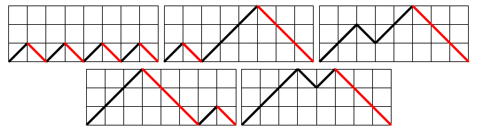
Dyck paths consist of up-steps \((1,1)\) and down-steps \((1,-1)\), are not allowed to go below the \(x\)-axis and end at the \(x\)-axis. The enumeration (path consisting of \(2n\) steps) is via the Catalan numbers \(\mathcal{C}_n=\frac1{n+1}\binom{2n}{n}\). Sometimes, paths that do not necessarily end at the \(x\)-axis are also called Dyck (Catalan) paths. The ultimate reference is Stanley’s book [1]. This book offers in Exercise 26 an interesting alternative: Maximal sequences of down-steps, when the end on the \(x\)-axis must always have odd length. This restriction leads to smaller numbers of paths, but interestingly restricted paths consisting of \(2n+2\) steps are also enumerated by Catalan numbers \(\mathcal{C}_n\). The 5 allowed paths of length 8 are depicted in Figure 1:

In the first of this paper we will enumerate prefixes of restricted paths à la Stanley: they can be completed to allowed paths. An alternative name of these combinatorial objects is partial Stanley-Dyck paths. We might also say that a maximal down-run the \(x\)-axis of even length has never occured in a partial Dyck path. The method of choice is generating functions (in \(z\) marking the length) but also in \(u\), marking the final level. The details will appear in the next section.

In the final section an additional restriction (skew Dyck paths) will be combined with the Stanley restriction: They allow an additional type of south-west step, but no overlap is allowed to occur. As in a previous publication [2] we prefer to draw a down-step \((1,-1)\) but depict it with the red color.

As in various examples discussed in the past [2, 3, 4] we will use the kernel method to set up appropriate generating functions. There are three bivariate generating functions \(F(u), G(u), H(u)\) (also depending on \(z\)) related to the nature of the last step of the prefix of a Stanley-Dyck path. To solve the system, a ‘bad’ factor \(u-r_2\) must be divided out from numerator and denominator, after which one can plug in \(u=0\) and identify the unknown quantities \(f_1=F(0)\), \(h_0=H(0)\). The function \(r_2(z)\) generates Catalan numbers.

In the final section, instead of 3 functions, we have to deal with 5 functions, but the strategy is similar. The function that plays the role of \(r_2\) now has coefficients 1, 3, 10, 36, 137, 543, 2219, 9285, 39587, 171369, 751236, which is sequence A2212 in [5]. The paper [4] contains a fair amount of combinatorics around this sequence.

2. Prefixes of Dyck Paths with Only Maximal Down-Runs to the\(x\)-axis of Odd Length

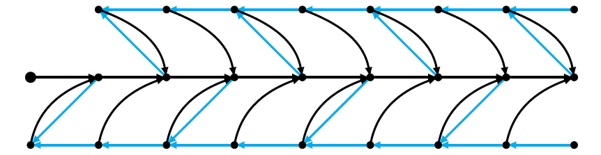
We present a graph that allows to identify all prefixes of Stanley-Dyck path. It has 3 layers of states, and maximal sequences of down-steps are depicted in blue. Parity plays a role: if such a sequence would lead to the \(x\)-axis after an even number of states, this is prohibited as such a state in the first layer is missing. Otherwise we introduce sequences \(f_i\), \(i\ge1\), \(g_i\), \(h_i\), \(i\ge0\). These quantities all depend on the variable \(z\) and describe generating functions of paths leading to a particular state. The state \(h_0\) is special, it is related to Stanley-Dyck paths.

We read off recursions and introduce bivariate generating functions \[F(u)=\sum_{i\ge1}f_iu^{i-1},\quad G(u)=\sum_{i\ge0}g_iu^{i},\quad H(u)=\sum_{i\ge0}h_iu^{i}.\] The recursions are according to the last symbol read. Firstly, \[\begin{aligned} f_i&=zf_{i+1}+[i\text{ odd}]zg_{i+1},\ i\ge1,\quad\text{and}\\ \sum_{i\ge1}f_iu^i&=\sum_{i\ge1}zf_{i+1}u^i+\sum_{i\ge1}[i\text{ odd}]zg_{i+1}u^i, \\ uF(u)&=zF(u)-zf_1+\frac zu\sum_{i\ge0}[i\text{ even}]g_{i}u^i-\frac zu, \\ uF(u)&=zF(u)-zf_1+\frac z{2u}G(u)+\frac z{2u}G(-u)-\frac zu. \end{aligned}\] Secondly, \[\begin{aligned} h_i&=zh_{i+1}+[i\text{ even}]zg_{i+1},\ i\ge0,\quad\text{and}\\ H(u)&=\frac zuH(u)-\frac zuh_0+\frac zu\sum_{i\ge1}[i\text{ odd}]g_{i}u^{i},\\ H(u)&=\frac zuH(u)-\frac zuh_0+\frac z{2u}G(u)-\frac z{2u}G(-u). \end{aligned}\] Thirdly \[\begin{aligned} g_{i+1}&=zf_i+zg_i+zh_i,\ i\ge1,\ g_1=z+zh_0,\ g_0=1,\quad\text{and}\\ \sum_{i\ge1}g_{i+1}u^i&=\sum_{i\ge1}zf_iu^i+\sum_{i\ge1}zg_iu^i+\sum_{i\ge1}zh_iu^i, \ g_1=z+zh_0,\ g_0=1,\\ \frac1u G(u)-\frac1u&=zuF(u)+zG(u)+zH(u). \end{aligned}\] The 3 equations can be solved: We start with the simplest function \[G(u)=\frac{z^2u^2f_1+z^2uh_0-u+z^2u+z}{z-u+zu^2};\] to get a form that leads to further developments, we factorize the denominator: \[z-u+zu^2=z(u-r_1)(u-r_2),\quad r_1=\frac{1+\sqrt{1-4z^2}}{2z},\quad r_2=\frac{1-\sqrt{1-4z^2}}{2z}.\] Dividing out the factor \(u-r_2\) from numerator and denominator, we find¹ \[G(u)=\frac{r_2z^2f_1+z^2h_0-1+z^2+z^2uf_1}{r_2z-1+zu},\quad\text{and}\quad G(0)=1=\frac{r_2z^2f_1+z^2h_0-1+z^2}{r_2z-1}.\] Using this for \(G(u)\) and \(G(-u)\), we get \[F(u)=\frac{\Xi}{2u(z-u+zu^2)(u-z)}\] with \(\Xi=z(-2zf_1u^3+z^2u^2f_1+zu^2G(-u)-2zu^2+2u^2f_1+z^2uh_0+z^2u-2zf_1u-uG(-u)+u+zG(-u)-z)\). Dividing out the factor \(u(u-z)(u-r_2)\) we find an attractive answer \[F(u)=\frac{z^3(1+uf_1)}{1-z^2-zr_2-z^2u^2}, \quad F(0)=f_1=\frac{z^3}{1-z^2-zr_2}=\frac{1-2z^2-\sqrt{1-4z^2}}{2z}=r_2-z.\] From the equation \(G(0)=1=\dfrac{r_2z^2f_1+z^2h_0-1+z^2}{r_2z-1}\), with the already known \(f_1\), we conclude \[h_0=\frac{1-\sqrt{1-4z^2}}{2}=zr_2=z^2\sum_{n\ge0} \mathcal{C}_nz^{2n}=\sum_{n\ge0} \mathcal{C}_nz^{2n+2},\] as predicted by Stanley [1]. Further simplifications include \[F(u)=\frac{z(\frac{r_2}{z}-1)(1+zu(\frac{r_2}{z}-1))}{1-(\frac{r_2}{z}-1)u^2}=\frac{(1+uzr_2^2)r_2^2}{1-r_2^2u^2},\] \[\begin{aligned} H(u)&=\frac{z^2(1-z^2+uzh_0-zf_1)}{1-z^2-r_2z-z^2u^2}\\ &=\frac{z^2(1-z^2+uz^2r_2-z(r_2-z))}{1-z^2-r_2z}\frac{1}{1-(\frac{r_2}{z}-1)u^2}=\frac{(1+uzr_2^2)zr_2}{1-r_2^2u^2} \end{aligned}\] and \[G(u)=\frac{1-uz^2r_2^3}{1-r_2u}.\] This allows the following expansions \[\begin{gathered} F(u)=\frac{(1+uzr_2^2)r_2^2}{1-r_2^2u^2} =\sum_{k\ge0}r_2^{2k+2}u^{2k}+z\sum_{k\ge0}r_2^{2k+4}u^{2k+1},\\ G(u)=\frac{1-uz^2r_2^3}{1-r_2u}=\sum_{k\ge0}r_2^ku^k-z^2\sum_{k\ge0}r_2^{k+3}u^{k+1},\\ H(u)=\frac{(1+uzr_2^2)zr_2}{1-r_2^2u^2}=z\sum_{k\ge0}r_2^{2k+1}u^{2k}+z^2\sum_{k\ge0}r_2^{2k+3}u^{2k+1}. \end{gathered}\] Classically, we know that \[r_2^j=z^j\sum_{n\ge0}\frac{j(2n+j-1)!}{n!(n+j)!}z^{2n}.\] Then \[f_j=[u^{j-1}]F(u)=\begin{cases}r_2^{j+1}& j\text{ odd},\\ zr_2^{j+2}& j\text{ even}. \end{cases}\] Further, \(g_0=1\) and for \(j\ge1\) \[g_j=r_2^j-z^2r_2^{j+2}.\] Finally, \[h_j=[u^j]z\sum_{k\ge0}r_2^{2k+1}u^{2k}+[u^j]z^2\sum_{k\ge0}r_2^{2k+3}u^{2k+1} =\begin{cases}z^2r_2^{j+2}& j\text{ odd},\\ zr_2^{j+1}& j\text{ even}. \end{cases}\]

An interesting quantity is \(F(1)+G(1)+H(1)\), which is the generating function of all prefixes of Stanley-Dyck paths, regardless of where they end; \[\begin{aligned} F(1)&+G(1)+H(1)=\frac{1-z}{2}+\frac12\frac{1+z}{1-2z}\sqrt{1-4z^2}\\ &=1+z+2z^2+3z^3+5z^4+9z^5+16z^6+30z^7+55z^8+105z^9+196z^{10}+378z^{11}+\dots\,. \end{aligned}\]

Remark. Stanley’s [1] exercise 31 is a variation due to Callan [6]. The last run to the \(x\)-axis must have even length, all others (if any) odd length.

This can be found by \(zf_1\), since the factor \(z\) stands for an extra down-step, making the final number of down-steps even. But \(zf_1=zr_2-z^2\) and \(h_0=zr_2\), so these series coincide except for a Dyck-path of length 2, as predicted and proved by Callan.

3. Skew Dyck Paths and the Stanley Restriction

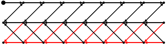
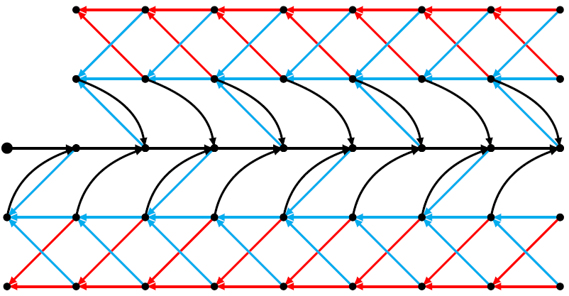
Skew Dyck paths [9] are augmented Dyck paths with additional south-west steps \((-1,-1)\), but no overlaps. In [2] we preferred to replace these extra steps by red down-steps; red-up resp. up-red are forbidden because of overlaps. The graph Figure 2 describes the allowed paths. If they end on level 0, they are skew Dyck paths, otherwise just prefixes of them.

The relevant recursions can be read off, again by considering a last step of a partial path. \[\begin{aligned} e_i&=ze_{i+1}+zf_{i+1}, i\ge1\\ f_i&=ze_{i+1}+zf_{i+1}+[i\text{ odd}]zg_{i+1}, i\ge1\\ g_{i+1}&=zf_i+zg_i+zh_i,\ i\ge1,\ g_1=z+zh_0,\ g_0=1\\ h_i&=zh_{i+1}+[i\text{ even}]zg_{i+1}+zk_{i+1},\ i\ge0\\ k_i&=zh_{i+1}+zk_{i+1},\ i\ge0. \end{aligned}\] Summing, \[\begin{aligned} \sum_{i\ge1}u^ie_i&=\sum_{i\ge1}u^ize_{i+1}+\sum_{i\ge1}u^izf_{i+1}\\ \frac uzE(u)&=E(u)-e_1+F(u)-f_1; \end{aligned}\] \[\begin{aligned} \sum_{i\ge1}u^if_i&=\sum_{i\ge1}u^ize_{i+1}+\sum_{i\ge1}u^izf_{i+1}+\sum_{i\ge1}u^i[i\text{ odd}]zg_{i+1}\\ \frac uzF(u)&=E(u)-e_1+F(u)-f_1+\frac1u\sum_{i\ge2}u^i[i\text{ even }]g_{i}\\ \frac uzF(u)&=E(u)-e_1+F(u)-f_1+\frac1{2u}G(u)+\frac1{2u}G(-u)-\frac1u; \end{aligned}\] \[\begin{aligned} g_1+\sum_{i\ge1}u^ig_{i+1}&=\sum_{i\ge1}u^izf_i+\sum_{i\ge1}u^izg_i+\sum_{i\ge1}u^izh_i+z+zh_0\\ \sum_{i\ge0}u^ig_{i+1}&=\sum_{i\ge1}u^izf_i+\sum_{i\ge0}u^izg_i+\sum_{i\ge0}u^izh_i\\ \frac{G(u)-1}{u}&=uzF(u)+zG(u)+zH(u); \end{aligned}\] \[\begin{aligned} \sum_{i\ge0}u^{i+1}h_i&=\sum_{i\ge0}u^{i+1}zh_{i+1}+\sum_{i\ge0}u^{i+1}[i\text{ even}]zg_{i+1}+\sum_{i\ge0}u^{i+1}zk_{i+1}\\ uH(u)&=z(H(u)-h_0)+z\sum_{i\ge1}u^{i}[i\text{ odd}]g_{i}+z(K(u)-k_0)\\ uH(u)&=z(H(u)-h_0)+\frac z2G(u)-\frac z2G(-u) +z(K(u)-k_0); \end{aligned}\] \[\begin{aligned} \sum_{i\ge0}u^{i+1}k_i&=\sum_{i\ge0}u^{i+1}zh_{i+1}+\sum_{i\ge0}u^{i+1}zk_{i+1}\\ uK(u)&=z(H(u)-h_0)+z(K(u)-k_0). \end{aligned}\] For convenience, we repeat the system that needs to be solved: \[\begin{aligned} \frac uzE(u)&=E(u)-e_1+F(u)-f_1,\\ \frac uzF(u)&=E(u)-e_1+F(u)-f_1+\frac1{2u}G(u)+\frac1{2u}G(-u)-\frac1u,\\ \frac{G(u)-1}{u}&=uzF(u)+zG(u)+zH(u),\\ uH(u)&=z(H(u)-h_0)+\frac z2G(u)-\frac z2G(-u) +z(K(u)-k_0),\\ uK(u)&=z(H(u)-h_0)+z(K(u)-k_0). \end{aligned}\] Again we start with the solution of the middle (simplest) function: \[G(u)=\frac {{z}^{2}{u}^{2}f_1+{z}^{2}{u}^{2}e_1+{z}^{2}u-u+{z}^{ 2}uh_0+{z}^{2}uk_0+2 z-{z}^{3}}{{u}^{2}z-u-{z}^{2}u+2 z-{z }^{3}}.\] The denominator is of interest, as one of the factor is ‘bad’: \[u^2z-u-z^2u+2z-z^3=z(u-r_1)(u-r_2),\] with \[r_1=\frac{1+z^2+\sqrt{1-6z^2+5z^4}}{2z},\quad r_2=\frac{1+z^2-\sqrt{1-6z^2+5z^4}}{2z}.\] Dividing out the factor \(u-r_2\), \[G(u)=\frac {{ r_2} {z}^{2}{ f_1}+{ r_2} {z}^{2}{ e_1}+{z}^ {2}-1+{z}^{2}{ h_0}+{z}^{2}{ k_0}+u{z}^{2}{ f_0}+u{z}^{2}{ e_1}}{{ r_2} z-1-{z}^{2}+zu},\] which is what we need. Dividing out \((u-r_2)(u-2z)u^2\) from the first two functions, \[E(u)=-{\frac { ( { f_1}+{ e_1} ) {z}^{3} ( u+2 z ) }{{r_2} z+{z}^{3}{r_2}+{z}^{2}{u}^{2}-1-2 {z}^{4}}}\] and \[F(u)=-{\frac {{z}^{3} ( u{ f_1}+u{ e_1}+1+{ f_1} z+{ e_1} z ) }{{ r_2} z+{z}^{3}{ r_2}+{z}^{2}{u}^{2}-1-2 {z}^{4}}}.\] Dividing out \((u-r_2)(u-2z)u\) from the last two functions, \[H(u)={\frac {{z}^{2} ( -uz{ k_0}-uz{ h_0}+{z}^{3}{ e_1}+{z}^{3}{ f_1}-{z}^{2}{ h_0}-{z}^{2}{ k_0}+{z}^{2}-1+{ f_1} z+{ e_1} z ) }{{r_2} z+{z}^{3}{r_2}+{z}^{2}{u}^{2}-1-2 {z}^{4}}}\] and \[K(u)=-{\frac {{z}^{3} ( { k_0}+{ h_0} ) ( u+2 z ) }{{r_2} z+{z}^{3}{r_2}+{z}^{2}{u}^{2}-1-2 {z}^{4}}}.\] Now we can insert \(u=0\) and solve: \[\begin{aligned} e_1&=-2 {\frac {{z}^{5}-3 {z}^{3}+2 r_2 {z}^{2}+2 z-r_2}{ ( 1+{z}^{2} ) ( -2+{z}^{2} ) ^{2}}},\\ f_1&={\frac {-4 z+2 r_2+r_2 {z}^{4}+2 {z}^{3}}{ ( 1+{z}^ {2} ) ( -2+{z}^{2} ) ^{2}}} ,\\ h_0&=-{\frac { ( {z}^{3}-2 z+2 r_2 ) z}{ ( -2+{z}^{2 } ) ( 1+{z}^{2} ) }} ,\\ k_0&=2 {\frac { ( -{z}^{3}+r_2 {z}^{2}+2 z-r_2 ) z} { ( -2+{z}^{2} ) ( 1+{z}^{2} ) }} . \end{aligned}\] This leads eventually to \[\begin{aligned} E(u)&={\frac { \left( r_2-2 z \right) {z}^{3} \left( u+2 z \right) } { \left( 1+{z}^{2} \right) (1+2 {z}^{4} -r_2 z-{z}^{3}r_2-{z}^{2}{u}^{2} ) }},\\ F(u)&=-{\frac { \left( r_2-2 z \right) \left( r_2 z+{z}^{3}{\it rw}-{z}^{3}u-1 \right) }{ \left( 1+{z}^{2} \right) (1+2 {z}^{4} -r_2 z-{z}^{3}r_2-{z}^{2}{u}^{2} )}},\\ G(u)&=-{\frac { \left( r_2-2 z \right) \left( r_2 {z}^{5}-2 {z }^{4}-{z}^{5}u-r_2 z-{z}^{2}+1 \right) }{{z}^{3} \left( 1+{z}^{2 } \right) \left( r_2 z-1-{z}^{2}+zu \right) }},\\ H(u)&=-{\frac { \left( r_2 z+{z}^{3}r_2-{z}^{3}u-1 \right) z \left( -3 z+2 r_2 \right) }{ \left( 1+{z}^{2} \right) (1+2 {z}^{4} -r_2 z-{z}^{3}r_2-{z}^{2}{u}^{2} )}},\\ K(u)&={\frac { \left( -3 z+2 r_2 \right) \left( u+2 z \right) {z}^ {4}}{ \left( 1+{z}^{2} \right) (1+2 {z}^{4} -r_2 z-{z}^{3}r_2-{z}^{2}{u}^{2} ) }} \end{aligned}\] and, which is useful for expansion, \[\begin{aligned} E(u)&=\frac{1}{(2-z^2)^2}{\frac { \left( r_2-2 z \right) {z} \left( u+2 z \right) } { \left( 1+{z}^{2} \right) \bigl(1-\frac{z^2r_2u^2}{(2-z^2)^2}\bigr) }},\\ F(u)&=\frac{1}{z^2(2-z^2)^2} \frac { \left( r_2-2 z \right) \left(1- r_2 z-{z}^{3}r_2+{z}^{3}u \right) }{ \left( 1+{z}^{2} \right) (1-\frac{z^2r_2u^2}{(2-z^2)^2})},\\ G(u)&={\frac { \left( r_2-2 z \right) \left( r_2 {z}^{5}-2 {z }^{4}-{z}^{5}u-r_2 z-{z}^{2}+1 \right) }{{z}^{3} \left( 1+{z}^{2 } \right) \left(1- r_2 z+{z}^{2}-zu \right) }},\\ H(u)&=\frac{1}{z(2-z^2)^2}{\frac { \left(1 -r_2 z-{z}^{3}r_2+{z}^{3}u \right) \left( -3 z+2 r_2 \right) }{ \left( 1+{z}^{2} \right) \bigl(1-\frac{z^2r_2u^2}{(2-z^2)^2}\bigr) }},\\ K(u)&=\frac{1}{(2-z^2)^2}{\frac { \left( -3 z+2 r_2 \right) \left( u+2 z \right) {z}^ {2}}{ \left( 1+{z}^{2} \right) \bigl(1-\frac{z^2r_2u^2}{(2-z^2)^2}\bigr) }}. \end{aligned}\] For the simplest function \(G(u)\) we show the decomposition in detail: \[\begin{aligned} G(u)&=1+\frac{zu(1+3z^2-zr_2)}{(1+z^2)(1+z^2-zr_2-zu)}\\ &=1+\frac{u(1+3z^2-zr_2)r_2}{(2-z^2)(1+z^2)\Bigl(1-\frac{r_2}{2-z^2}u\Bigr)}\\ &=1+\sum_{k\ge1}\Big(\frac{r_2}{2-z^2}\Big)^ku^k \frac{(1+3z^2-zr_2)}{(1+z^2)}. \end{aligned}\]

Again we can compute the total generating function of paths, regardless where they end: \[\begin{aligned} E(1)+F(1)&+G(1)+H(1)+K(1)\\* &=\frac{z(2z^3+9z^2+4z-7)+(z+2)(2z+1)\sqrt{1-6z^2+5z^4}}{2(1+z^2)(1-2z-z^2)}\\ &=1+z+2z^2+3z^3+5z^4+10z^5+20z^6+38z^7+75z^8+150z^9+ \dots\,. \end{aligned}\]

The Coefficients of \(r_2\).

We report here briefly how to compute the coefficients of \[r_2^{\ell}=z^\ell\Big(\frac {r_2}{z}\Big)^\ell=z^\ell\bigg(\frac{1+Z-\sqrt{1-6Z+5Z^2}}{2Z}\bigg)^\ell,\] with \(Z=z^2\). As in [4], we set \(Z=\dfrac{v}{1+3v+v^2}\), so that \(\frac{r_2}{z}=2+v\). Then \[\begin{aligned} r_2^{\ell}&=\frac1{2\pi i}\oint \frac{dZ}{Z^{n+1}}(2+v)^\ell\\ &=\frac1{2\pi i}\oint \frac{dv(1-v^2)}{(1+3v+v^2)^{2}}\frac{(1+3v+v^2)^{n+1}}{v^{n+1}}(2+v)^\ell\\ &=[v^n](1-v^2)(1+3v+v^2)^{N-1}\sum_{k=0}^\ell\binom{\ell}{k}2^{\ell-k}v^k\\ &=\sum_{k=0}^\ell\binom{\ell}{k}2^{\ell-k}[v^{n-k}](1-v^2)(1+3v+v^2)^{n-1}\\ &=\sum_{k=0}^\ell\binom{\ell}{k}2^{\ell-k}\biggl[\binom{n-1;1,3,1}{n-k}-\binom{n-1;1,3,1}{n-k-2}\biggr], \end{aligned}\] with weighted trinomial coefficients \(\dbinom{n;1,3,1}{k}:=[t^k](1+3t+t^2)^n\).

Conflict of Interest

All author declares that they have no conflicts of interest.