Total coloring and efficient domination applications to non-cayley non-shreier vertex-transitive graphs

1. Efficient domination and total coloring of graphs

Let $0<k\in \mathbb{Z}$. Given a finite graph $G=(V(G),E(G))$ and a subset $S\subseteq V(G)$, it is said that $S$ is an efficient dominating set (E-set) [1,3,2,6,7,10] or a perfect code [4,5], if for each $v\in V(G)\setminus S$ there exists exactly one vertex $v^0$ in $S$ such that $v$ is adjacent to $v^0$.

Applications of E-sets occur in: (a) the theory of error-correcting codes and (b) establishing the existence of regular graphs for Network Theory by removing E-sets from their containing graphs.

A total coloring of a graph $G$ is an assignment of colors to the vertices and edges of $G$ such that no two incident or adjacent elements (vertices or edges) are assigned the same color [8]. A total coloring of $G$ such that the vertices adjacent to each $v\in V(G)$ together with $v$ itself are assigned pairwise different colors will be said to be an efficient coloring. The efficient coloring will be said to be totally efficient if $G$ is $k$-regular, the color set is $[k]=\{0,1,\dots ,k-1\}$ and each $v\in V(G)$ together with its neighbors are assigned all the colors in $[k]$. The total (resp. efficient) chromatic number ${\chi }^{″}(G)$ (resp. ${\chi }^{‴}(G)$) of $G$ is defined as the least number of colors required by a total (resp. efficient) coloring of $G$.

As for applications other than (a)-(b) above, note that: (c) by removing the vertices of a fixed color, then again regular graphs for Network Theory are generated; (d) by removing the edges of a fixed color, then copies of a non-bipartite biregular graph whose parts have vertices with degrees differing in a unit are determined, again applicable in Network Theory.

In Section 3, we show that the graphs of a family of graphs $G=S{T}_k^2$, ($0<k\in \mathbb{Z}$), introduced in Section 2, satisfy the conditions of the following theorem. We conjecture that those conditions are only satisfied by such graphs $G=S{T}_k^2$, and not any other graphs.

Let $\ell \in \{0,1\}$. In Section 5, we generalize via $\ell$-set permutations, (see Section 2), the result of [6] that the star transposition graphs form a dense segmental neighborly E-chain. In Section 6, we generalize star transposition graphs to pancake transposition graphs and related intermediate graphs [6], leading to an adequate version of dense neighborly E-chain [6], with obstructions preventing any convenient version of segmental E-chain [6].

2. Families of multiset transposition graphs with E-sets

Let $0<\ell \in \mathbb{Z}$ and let $1<k\in \mathbb{Z}$. We say that a string over the alphabet $[k]$ that contains exactly $\ell$ occurrences of $i$, for each $i\in [k]$, is an $\ell$–set permutation. In denoting specific $\ell$-set permutations, commas and brackets are often omitted.

Let $V_k^{\ell }$ be the set of all $\ell$-set permutations of length $k\ell$. Let the star $\ell$-set transposition graph $S{T}_k^{\ell }$ be the graph on vertex set $V_k^{\ell }$ with an edge between each two vertices $v=v_0{v}_1\cdots v_{k\ell -1}$ and $w=w_0{w}_1\cdots w_{k\ell -1}$ that differ in a star transposition, i.e. by swapping the first entry $v_0$ of $v=v_0{v}_1\cdots v_{k\ell -1}\in V_k^{\ell }$ with any entry $v_j$ ($j\in [k\ell ]\setminus \{0\}$) whose value differs from that of $v_0$ (so $v_j\ne v_0$), thus obtaining either $w=w_0\cdots w_j\cdots w_{k\ell -1}=v_j\cdots v_0\cdots w_{k\ell -1}$ or $w=w_0\cdots w_{k\ell -1}=v_{k\ell -1}\cdots v_0$. In other words, each edge of $S{T}_k^{\ell }$ is given by the transposition of the initial entry of an endvertex string with an entry that contains a different symbol than that of the initial entry. The graphs $S{T}_k^{\ell }$ are a particular case of the graphs treated in [9] in a context of determination of Hamilton cycles.

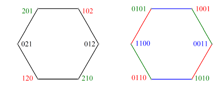
It is known that all $k$-permutations, (that is all 1-set permutations of length $k$), form the symmetric group, denoted $Sy{m}_k$, under composition of $k$-permutations, each $k$-permutation $v_0{v}_1\cdots v_{k-1}$ taken as a bijection from the identity $k$-permutation $01\cdots (k-1)$ onto $v_0{v}_1\cdot v_{k-1}$ itself. A graph $S{T}_k^1$ with $k>1$ (which excludes $S{T}_1^1$) is the Cayley graph of $Sy{m}_k$ with respect to the set of transpositions $\{(0i);i\in [k]\setminus \{0\}\}$. Such a graph is denoted $S{T}_k$ in [1,6], where is proven its vertex set admits a partition into $k$ E-sets, exemplified on the left of Figure 1 for $S{T}_3^1=S{T}_3$, with the vertex parts of the partition differentially colored in black, red and green, for respective first entries 0, 1 and 2. Figure 1 of [6] shows a similar example for $S{T}_4^1=S{T}_4$. Also, the graph $S{T}_k^{\ell }$ is vertex transitive, but is neither a Cayley graph nor a Shreier graph; see Subsection 5.1, below.

3. E-sets of star 2-set transposition graphs

Let $i\in [2k]\setminus \{0\}=\{1,\dots ,2k-1\}$. Let ${\mathrm{\Sigma }}_i^k$ be the set of vertices $v_0{v}_1\cdots v_{k\ell -1}$ of $S{T}_k^{\ell }$ such that $v_0=v_i$, ($i=1,\dots ,2k-1$). Let $E_i^k$ be the set of edges having color $i$ in $G\setminus {\mathrm{\Sigma }}_i^k$. We will show that ${\mathrm{\Sigma }}_i^k$ is an E-set of $S{T}_k^2$. Clearly, no edge of $E_i^k$ is incident to the vertices of ${\mathrm{\Sigma }}_i^k$.

Example 3.4. The graph $S{T}_3^2$ has the E-set ${\mathrm{\Sigma }}_5^3$ with 18 vertices denoted as in display (1): $$\begin{array}{}\text{(1)}& \begin{array}{r}\{\begin{array}{cccccc}A=011220,& \underset{\_}{A}=022110,& B=012210,& \underset{\_}{B}=021120,& C=012120,& \underset{\_}{C}=021210,\\ D=122001,& \underset{\_}{D}=100221,& E=120021,& \underset{\_}{E}=102201,& F=120201,& \underset{\_}{F}=102021,\\ G=200112,& \underset{\_}{G}=211002,& H=201102,& \underset{\_}{H}=210012,& J=201012,& \underset{\_}{J}=210102.\end{array}\end{array}\end{array}$$

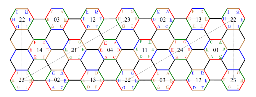
A planar interconnected disposition of the 6-cycles of the subgraph $S{T}_3^2\setminus {\mathrm{\Sigma }}_5^3$ of $S{T}_3^2$ is shown in Figure 2. The edges of such 6-cycles are alternatively colored with 2 or 3 colors of the color form $(ababab)$ or $(abcabc)$ respectively, where $\{a,b,c\}\subseteq \{1,2,3,4\}$ is a subset of colors provided by the respective positions 1,2,3,4 of the $6$-tuples taken as the vertices of $S{T}_3^2$.

The tessellation suggested in Figure 2 can be extended to the whole plane as an unfolding of the fundamental region delimited by the shown dash-border rectangle – call it $R$. This $R$ appears partitioned via dashed segments into two right triangles and a rhomboid in between. By transporting the left right triangle – call it $T_l\subset R$ – to a new position $T_l^{\prime }$ to the right so that the vertical side of $T_l^{\prime }$ coincides with the right side of $R$, a rhomboid $R^{\prime }$ is obtained. Identification of the tilted sides of $R^{\prime }$ and of its horizontal sides allows to view a toroidal embedding of $S{T}_3^2\setminus {\mathrm{\Sigma }}_5^3$.

Edge colors in Figure 2 are numbered as follows (indicating corresponding subsequent positions in the 6-tuples representing the vertices of $S{T}_3^2$): $$\begin{array}{}\text{(2)}& \begin{array}{r}1=green,2=blue,3=hazel,4=red,5=black.\end{array}\end{array}$$

In Figure 2, the 3-colored 6-cycles are exactly those containing in their interiors (next to their corresponding denoting vertices) the (possibly underlined) capital letters of display (1), but each such letter colored as indicated in display (2). Each such number color $a\in \{1,2,3,4\}$ as in display (2) of a symbol $X\in \{A,\dots ,J,\underset{\_}{A},\dots ,\underset{\_}{J}\}$ in Figure 2 indicates the existence of an (absent) $a$-colored edge between $V_3^2\setminus {\mathrm{\Sigma }}_5^3$ and ${\mathrm{\Sigma }}_5^3$ in $S{T}_3^2$. Figure 3 shows each such edge in exactly one copy $\mathrm{{\rm Y}}$ of $K_{1,4}$ with its endvertex in ${\mathrm{\Sigma }}_5^3$ represented by $X$ (in black) and its other endvertex being the sole element of $\mathrm{{\rm Y}}\cap V_3^2\setminus {\mathrm{\Sigma }}_5^3$, namely the $a$-colored $X$, that we denote as $X^a$ in Table 1. In fact, Table 1 reproduces the data of Figure 2 in a likewise disposition, with the vertex notation $X^a$ instead of the $a$-colored $X$ notation of Figure 2. In Table 1, edges are represented by their numeric symbols (display (2)) and appear interspersed with the symbols $X^a$ in representing the 3-colored 6-cycles, while 2-colored 6-cycles are represented by the disposition of their numeric symbols. Note in Figure 2 that each 3-colored 6-cycle is bordered by six 2-colored 6-cycles via edges colored in $\{1,2,3,4,\}$, while each 2-colored 6-cycle, call it $\mathrm{\Theta }$, is bordered by three 3-colored 6-cycles (via edges in one fixed color of $\{1,2,3,4\}$) alternated with three 2-colored 6-cycles via an edge matching bordering $\mathrm{\Theta }$ and whose color is 1.

Table 2 represents the twelve 3-colored 6-cycles, as follows. The six centers $X\in \{A,\dots ,J,$ $\underset{\_}{A},\dots ,\underset{\_}{J}\}$ of copies of $K_{1,4}$ involved with one such 3-colored 6-cycle, call it $\mathrm{\Phi }$, are represented by 6-tuples that are expressed in Table 2 in a 6-row section of a column whose heading is ${\mathrm{\Sigma }}_5^3$. To the immediate right of each such 6-row section, another 6-row section of 6-tuples expresses the corresponding neighbors $X^b$, for a fixed color $b\in \{1,2,3,4\}$, via $b$-colored edges. Such neighbors $X^b$ conform $V(\mathrm{\Phi })$ and induce $\mathrm{\Phi }$. In fact, Table 2 contains the twelve instances of such representations.

Notice that the vertices in display (1) are of the form $i{a}_1{a}_2{a}_3{a}_{4}i$. Centered inside each 3-colored 6-cycle $\mathrm{\Phi }$ in Figure 2, a pair $(i,b)$ of digits (written as $ib$) indicates the fixed double entry $i\in \{0,1,2\}$ of the vertices $i{a}_1{a}_2{a}_3{a}_{4}i$ of ${\mathrm{\Sigma }}_5^3$ in $\mathrm{\Phi }$ and the fixed color $b$ their representing symbols have in the figure.

To facilitate viewing the edge colors along each $\mathrm{\Phi }$, the second row in Table 2 shows the 6-tuple $x$ of subsequent positions (or colors), $012345$, of the 6-tuples representing each $X$ and $X^b$. In each such $x$ under the heading ${\mathrm{\Sigma }}_5^3$, the entry $b\in \{1,2,3,4\}$ of the corresponding $X^b$ is underlined, while under each subsequent heading $X^b$, the other three entries in $\{1,2,3,4\}$ are underlined to indicate the entries successively transposed with the initial entry in the subsequent vertically disposed 6-tuples of each particular $\mathrm{\Phi }$.

Observe the difference between 3-colored 6-cycles appearing here and 2-colored 6-cycles in that the former are created by transpositions not involving the initial entry while the latter do involve transpositions with the initial entry.

In Figure 2, deletion of the edges colored 1 from $S{T}_3^2\setminus {\mathrm{\Sigma }}_5^3$ leaves a subgraph with twelve components, each being a 3-colored 6-cycle. Note that $E(S{T}_3^2)$ has a 1-factorization into five 1-factors $E_1^3,E_2^3,E_3^3,E_4^3,E_5^3$, each $E_i^3$ composed by those edges colored $i$, ($i\in [6]\setminus \{0\}$). Moreover, $S{T}_3^2\setminus {\mathrm{\Sigma }}_5^3\setminus E_5^3$ is the union of the twelve 3-colored 6-cycles in Table 2.

A characterization of the twenty-four 2-colored 6-cycles of $S{T}_3^2\setminus {\mathrm{\Sigma }}_1^3$ is also available from that of the twelve 3-colored 6-cycles in display (3). Let us observe the triple $(0x_0,1y_1,2y_2)$ formed by the three pairs $0x_0$, $1x_1$, $2x_2$ denoting the three 3-colored 6-cycles that share each an edge $e$ with a given 2-colored 6-cycle ${\mathrm{\Theta }}_e$. By shortening each such triple of pairs to the triple of colors $x_0{x}_1{x}_2$ and setting its missing color $x_3$ in $\{1,2,3,4\}$ as a subindex, with colors $i=5$ and $x_3$ assigned alternatively to the edges of each ${\mathrm{\Theta }}_e$, we have now the disposition in display (4) which is similar to that of Figure 2: $$\begin{array}{}\text{(4)}& \begin{array}{r}\begin{array}{ccccccccccccc}22& & 03& & 12& & 23& & 02& & 13& & 22\\ {142}_3& {342}_1& {341}_2& {321}_4& {421}_3& {423}_1& {413}_2& {213}_4& {214}_3& {234}_1& {134}_2& {132}_4& {142}_3\\ & 14& & 21& & 04& & 11& & 24& & 01& \\ {143}_2& {243}_1& {241}_3& {231}_4& {431}_2& {432}_1& {412}_3& {312}_4& {314}_2& {324}_1& {124}_3& {123}_4& {143}_2\\ 23& & 02& & 13& & 22& & 03& & 12& & 23\end{array}\end{array}\end{array}$$

Again, this disposition is encoded as $(123,1234)$.

4. Open problems

We conjectured that the graph $G$ in the statement of Theorem 1.1 must necessarily coincide with some $S{T}_k^2$. On the other hand, the twenty-four 2-colored 6-cycles of $S{T}_3^2\setminus {\mathrm{\Sigma }}_5^3$ generalize to 2-colored 6-cycles in $S{T}_k^2\setminus {\mathrm{\Sigma }}_{2k-1}^k$, for any $k>3$, by similarly alternating three black edges (meaning color $2k-1$) with three edges of a common color different from $2k-1$ in order to obtain one such 2-colored 6-cycle. Performing this to include all edges of $S{T}_k^2\setminus {\mathrm{\Sigma }}_{2k-1}^k$, still we do not know how to generalize for $k>3$ what happens between the $k{2}^{k-1}$ copies of $S{T}_{k-1}^2$ in Theorem 3.1 and the black edges (colored via $2k-1$). The determination of this particular matter is left as an open problem.

As a hint to illuminate the problem, let us recall that $S{T}_k^2$ has $\frac{(2k)!}{2^k}$ vertices and regular degree $2(k-1)$; then it has $\frac{(2k)!(k-1)}{2^k}$ edges and a total coloring via $2k-1$ colors. The number of vertices in $S{T}_k^2$ having a fixed color is $\frac{(2k)!}{2^k(2k-1)}$. The copies of stars $K_{1,2k-2}$ with centers on vertices of $S{T}_k^2$ having a fixed color contain a total of $\frac{(2k)!(2k-2)}{2^k(2k-1)}=\frac{2k)!(k-1)}{2^{k-1}(2k-1)}$ edges. The numbers of remaining vertices and edges, namely those of $S{T}_k^2\setminus {\mathrm{\Sigma }}_{2k-1}^k$, are $\frac{(2k)!}{2^k}-\frac{(2k)!}{2^k(2k-1)}$ and $\frac{(2k)!(2k-1)}{2^k}-\frac{(2k)!(k-1)}{2^{k-1}(2k-1)}$, respectively. The edges of $S{T}_k^2\setminus {\mathrm{\Sigma }}_{2k-1}^k$ with a fixed color are divided into groups of three edges, each such group with alternate edges of a corresponding 2-colored 6-cycle, with the other three alternating edges in color $2k-1$. A conclusion here is that the number of 2-colored 6-cycles must be the third part of $\frac{(2k)!(2k-1)}{2^k}-\frac{(2k)!(k-1)}{2^{k-1}(2k-1)}$, which for $k=3$ equals 24, as can be counted for example via Figure 2.

5. Conclusions for star 2-set transposition graphs

Let us recall from [6] that:

1. a countable family of graphs $$\mathcal{G}=\{{\mathrm{\Gamma }}_1\subset {\mathrm{\Gamma }}_2\subset \cdots \subset {\mathrm{\Gamma }}_i\subset {\mathrm{\Gamma }}_{i+1}\subset \cdots \},$$ is said to be an E-chain if every ${\mathrm{\Gamma }}_i$ is an induced subgraph of ${\mathrm{\Gamma }}_{i+1}$ and each ${\mathrm{\Gamma }}_i$ has an E-set $C_i$;

2. for graphs $\mathrm{\Gamma }$ and ${\mathrm{\Gamma }}^{\prime }$, a one-to-one graph homomorphism $\zeta :\mathrm{\Gamma }\to {\mathrm{\Gamma }}^{\prime }$ such that $\zeta (\mathrm{\Gamma })$ is an induced subgraph of ${\mathrm{\Gamma }}^{\prime }$ is said to be an inclusive map;

3. for $i\ge 1$, let ${\kappa }_i$ be an inclusive map of ${\mathrm{\Gamma }}_i$ into ${\mathrm{\Gamma }}_{i+1}$; if $C_{i+1}=N({\kappa }_i(V({\mathrm{\Gamma }}_i)))$, then the E-chain $\mathcal{G}$ is said to be a neighborly E-chain;

4. a particular case of E-chain $\mathcal{G}$ is the one in which $C_{i+1}$ has a partition into images ${\zeta }_i^{(j)}(C_i)$ of $C_i$ through respective inclusive maps ${\zeta }_i^{(j)}$, where $j$ varies on a suitable finite indexing set. In such a case, the E-chain is said to be segmental.

The notion of neighborly E-chain in item 3 above is not suitable in our context of graphs $S{T}_k^2$ and their E-sets, that we denote ${\mathrm{\Sigma }}_{2k-1}^k$ (instead of $C_i$ as in [6]), like ${\mathrm{\Sigma }}_3^2$ and ${\mathrm{\Sigma }}_5^3$ in Example 3.4, with ${\mathrm{\Sigma }}_5^3$ detailed both in display (1) and Figures 2-3, and also in Tables 1-2. In this context, the graphs $S{T}_k^2$ form an E-chain $$\begin{array}{}\text{(5)}& \begin{array}{r}\mathcal{S}\mathcal{T}(2)=\{S{T}_1^2\subset S{T}_2^2\subset \cdots \subset S{T}_k^2\subset S{T}_{k+1}^2\subset \cdots \},\end{array}\end{array}$$ with each inclusion $S{T}_k^2\subset S{T}_{k+1}^2$ realized by a set of $k+1$ neighborly maps $$\begin{array}{}\text{(6)}& \begin{array}{r}{\kappa }_k^j:S{T}_k^2\to S{T}_{k+1}^2,\end{array}\end{array}$$ ($j\in [k+1]$), (neighborly meaning that the images ${\kappa }_k^j(S{T}_i^2)$ are pairwise disjoint in $S{T}_{k+1}^2$ and that $$\begin{array}{}\text{(7)}& \begin{array}{r}{\mathrm{\Sigma }}_k^{k+1}={\cup }_{j=1}^{k-1}N({\kappa }_i^j(V_i^2)),\end{array}\end{array}$$ as a disjoint union), these neighborly maps given by $$\begin{array}{}\text{(8)}& \begin{array}{r}{\kappa }_k^j(a_0{a}_1\cdots a_{2k-2}{a}_{2k-1})=(a_0^j{a}_1^j\cdots a_{2k-2}^j{a}_{2k-1}^{j}jj),\end{array}\end{array}$$ for $j\in [k+1]$, where $$\begin{array}{}\text{(9)}& \begin{array}{r}{a}_i^k=a_i,a_i^{k+1}=a_i+1\mathrm{mod}(k+1),\dots ,a_i^{k+h}=a_i+h\mathrm{mod}(k+1),\dots ,\end{array}\end{array}$$ for $i=0.1,\dots ,2k-1$, the superindices $k+h$ of the entries $a_j^{k+h}$ taken mod $k+1$.

As an example, the last column of Table 2 offers disjoint neighborly maps ${\kappa }_2^j$, for $j=0,1,2$, yielding respectively the following images of the 6-cycle that comprises $S{T}_2^2$: $$\begin{array}{c}{\kappa }_2^2(1001,0011,1010,0110,1100,0101)=(100122,001122,101022,011022,110022,010122);\\ {\kappa }_2^0(1001,0011,1010,0110,1100,0101)=(211200,112200,212100,122100,221100,121200);\\ {\kappa }_2^1(1001,0011,1010,0110,1100,0101)=(022011,220011,020211,200211,002211,202011).\end{array}$$

An E-chain as in display (5) where each inclusion $S{T}_k^2\subset S{T}_{k+1}^2$ is realized by $k+1$ neighborly maps ${\kappa }_k^j$, as defined in displays (6) to (9), is said to be a disjoint neighborly E-chain.

The notion of segmental E-chain can also be generalized to the case of the graphs $S{T}_k^2$, where in item 3 above we replace “neighborly” by “disjoint neighborly”. In that case, the E-chain will be said to be disjoint segmental. It is clear by symmetry that the E-chain $\mathcal{S}\mathcal{T}(2)$ of display (5) is disjoint segmental, as exemplified via Figures 2 and 3 and the related Tables 1 and 2.

If, for each $i\ge 1$, there exists an inclusive map ${\zeta }_i:{\mathrm{\Gamma }}_i\to {\mathrm{\Gamma }}_{i+1}$ such that $\zeta (C_i)\subset C_{i+1}$, then [6] calls the E-chain inclusive and observes that an inclusive neighborly E-chain has ${\kappa }_i\ne {\zeta }_i$, for every positive integer $i$.

5.1. Density

In addition, [6] calls an E-chain $\mathcal{G}$ dense if, for each $n\ge 1$, one has $|V({\mathrm{\Gamma }}_n)|=(n+1)!$ and $|C_n|=n!$. However, this notion is not helpful in our present context.

For $k>1$, note that $S{T}_{k\ell }^1$ is the Cayley graph of $Sy{m}_{k\ell }$ generated by the transpositions $(0i)$, ($0<i<k\ell )$, but that $S{T}_k^{\ell }$ is not even a Shreier coset graph of the quotient of $Sy{m}_{k\ell }$ modulo say its subgroup $H_{\ell }$ generated by the transpositions $(aa+1)$, ($0\le a<k$), because the edges of $S{T}_k^{\ell }$ are not given by transpositions $(0i)$ independently of the values $i$ in different vertices of $S{T}_k^{\ell }$. However, Table 3 do generalize for every $S{T}_k^2$, ($k\ge 2$), where the table shows vertically:

1. the right cosets of $V_4^1$ mod the subgroup generated by transpositions $(01),(23)$;

2. the representations of such right cosets as vertices of $S{T}_2^2$; and

3. assigned generating sets of transpositions $(0i)$ per shown right coset of $V_3^1$ or its representing vertex in $S{T}_2^2$.

Tables like Table 3, but for $k>2$, suggest extending the definition of a Shreier coset graph as follows: A Shreier local coset graph of a group $G$, a subgroup $H$ of $G$ and a generating set $S(Hg)$ for each right coset $Hg$ of $H$ in $G$, is a graph whose vertices are the right cosets $Hg$ and whose edges are of the form $(Hg,Hgs)$, for $g\in G$ and $s\in S(Hg)$. The example in display (3) shows that $S{T}_2^2$ is a Shreier local coset graph of the group $V_4^1$, its subgroup $H$ generated by the transpositions $(01)$ and $(23)$, and the local generators indicated in the last line of the display. In a similar way, it can be shown for $k>2$ that $S{T}_k^2$ is a Shreier local coset graph of $V_k^2$ with respect to its subgroup generated by the transpositions $(2a2a+1)$ with $0\le a<k$. Now, the density observed in [6] must be replaced to be useful in the present context of 2-set star transposition graphs. It is clear that in this sense, the E-sets found in the graphs $S{T}_k^2$ in Section 3 are as dense as they can be, so we say that these E-sets are 2-dense. Then, the final conclusion of the present section is the following result.

6. Pancake 2-set transposition graphs

Let ${\pi }_i$ be an arbitrary product of independent transpositions on the set $\{1,\dots ,i-1\}$, ($i>1$), where ${\pi }_1$ and ${\pi }_2$ are the identity. For each integer $k\ge 1$, let $$A({\pi }_1,\dots ,{\pi }_i,\dots ,{\pi }_{2k-1})=\{(01){\pi }_1,\dots ,(0i){\pi }_i,\dots ,(0(2k-1)){\pi }_{2k-1}\}.$$

Lemma 2 of [6] implies that for $k\ge 1$ and any choice of the involutions ${\pi }_i$, ($i\ge 3$), the set $A({\pi }_1,\dots ,{\pi }_{2k-1})$ generates $Sy{m}_{2k-1}$. For each choice of involutions ${\pi }_1,{\pi }_2,\dots$, the sequence of Cayley graphs with generating set $A({\pi }_1,\dots ,{\pi }_{2k-1})$ forms a chain of nested graphs with natural inclusions ${\mathrm{\Gamma }}_k\subset {\mathrm{\Gamma }}_{k+1}$.

Let $\ell \in \{1,2\}$. If we choose the identity for each entry in $A({\pi }_1,\dots ,{\pi }_{2k-1})$, then we get the $\ell$-set star transposition graphs $S{T}_k^{\ell }$. If ${\pi }_i=(1(i-1))\cdots (\lfloor i/2\rfloor \lceil i/2\rceil )$, for $i=3,\dots ,k-1$, then we get the pancake $\ell$-set transpostion graph $P{C}_k^{\ell }$. In particular, the pancake 2-set transposition graph $P{C}_k^2$ has the same vertex set of $S{T}_k^2$ and its edges involve each the maximal product of concentric disjoint transpositions in any prefix of an endvertex string, including the external transposition being that of an edge of $S{T}_k^2$. The graphs $P{C}_k^1$ were seen in [6] to form a dense segmental neighborly E-chain $\mathcal{P}\mathcal{C}(1)=\{P{C}_1^1,P{C}_2^1,\dots ,P{C}_k^1,\dots \}$. (Figure 2 of [6] represents the graph $P{C}_4^1$). In a similar fashion to that of Section 5, the following partial extension of that result can be established.