
The Littlewood-Richardson coefficients appear in many areas of mathematics [5,8,9, 12,17]. An example comes from the study of symmetric functions. The set of Schur functions \(s_\lambda\), indexed by partitions \(\lambda\), is a linear basis for the ring of symmetric functions. Thus, for any partitions \(\lambda\) and \(\mu\), the product of Schur functions \(s_\lambda\) and \(s_\mu\) can be uniquely expressed as \[\begin{aligned} \label{eq:1} s_\lambda\cdot s_\mu = \sum_{\nu: |\nu| = |\lambda| + |\mu| } c^\nu_{\lambda,\mu} s_\nu, \end{aligned}\tag{1}\] for some real numbers \(c^\nu_{\lambda,\mu}\), where \(|\lambda|\) denotes the sum of the parts of \(\lambda\). The coefficient \(c^\nu_{\lambda,\mu}\) of \(s_\nu\) in (1) is called the Littlewood-Richardson coefficient.
There are several ways to compute \(c^\nu_{\lambda,\mu}\) such as the Littlewood-Richardson rule [14], the Littlewood-Richardson triangles [10], the Berenstein-Zelevinsky triangles [1], and the honeycombs [7]. In this paper, we employ the hive model that was first introduced by Knutson and Tao [7]. The hive model imposes certain inequalities that allow us to compute \(c^\nu_{\lambda,\mu}\) as the number of integer points in a rational polytope, which we call a hive polytope.
For fixed partitions \(\lambda, \mu, \nu\) such that \(|\nu| = |\lambda| + |\mu|\), we define the stretched Littlewood-Richardson coefficients to be the function \(c^{t\nu}_{t\lambda,t\mu}\) for non-negative integers \(t.\) The hive model implies that \[\begin{aligned} c^{t\nu}_{t\lambda,t\mu} = \text{ the number of integer points in the } t^{\mathrm{th}} \text{-dilation of the hive polytope}. \end{aligned}\]
By Ehrhart theory (see Thoerem 2.1), \(c^{t\nu}_{t\lambda,t\mu}\) is a quasi-polynolmial in \(t \in \mathbb{Z}\), which means \(c^{t\nu}_{t\lambda,t\mu}\) is a function of the form \(a_d(t)t^d + \cdots + a_1(t)t + a_0(t)\) where each of \(a_d(t), \dots, a_0(t)\) is a periodic function in \(t\) with an integral period. The function \(c^{t\nu}_{t\lambda,t\mu}\) was, however, observed and conjectured by King, Tollu, and Toumazet [6] to be a polynomial function in \(t\) (as opposed to a quasi-polynomial). The conjecture was then shown to be true by Derksen-Weyman [3], and Rassart [11]. More precisely, they proved the following theorem.
Theorem 1.1. Let \(\mu, \lambda, \nu\) be partitions with at most \(k\) part such that \(|\nu| = |\lambda| + |\mu|.\) Then \(c^{t\nu}_{t\lambda,t\mu}\) is a polynomial in \(t\) of degree at most \(\binom{k-1}{2}.\)
The proof by Derksen and Weyman [3] makes use of semi-invariants of quivers. They proved a result on the structure of a ring of quivers and then derived the polynomiality of \(c^{t\nu}_{t\lambda,t\mu}\) as a special case. Later, Rassart [11] proved a stronger result, which gives Theorem 1.1 as an easy consequence, by showing that \(c^{\nu}_{\lambda,\mu}\) is a polynomial in variables \(\lambda, \mu, \nu\) provided that they lie in certain polyhedral cones of a chamber complex. The proof by Rassart employs Steinberg’s formula, the hive conditions, and the Kostant partition function to give the chamber complex of cones in which \(c^{\nu}_{\lambda,\mu}\) is a polynomial in variables \(\lambda, \mu, \nu\). A considerably large portion of Rassart’s paper was devoted to describing this chamber complex and showing its desired property, resulting in a fairly long justification. We note that although this chamber complex of cones was provided, it is in practice computationally hard to work out the cones.
Inspired by Rassart’s approach, we ask if similar tools can be utilized to give a simple proof of Theorem 1.1 directly. We found that Steinberg’s formula and a simple argument about the chamber complex of the Kostant partition function are indeed sufficient. The main objective of this paper is to give a short alternative proof of Theorem 1.1 using this idea.
We begin this section by presenting necessary notations and theories related to polytopes and then describe the hive model for computing \(c^{\nu}_{\lambda,\mu}\). The hive model will help us understand the behavior of the stretched Littlewood-Richardson coefficients through a property of polytopes. We then introduce the Kostant partition functions and state Steinberg’s formula and related results that will later be used for proving Theorem 1.1.
A polyhedron \(P\) in \(\mathbb{R}^d\) is the solution to a finite set of linear inequalities, that is, \[P = \left\{(x_1, \dots, x_d) \in \mathbb{R}^d\,\Big\vert\, \sum^d_{j = 1}a_{ij}x_j \leq b_i \text{ for } i \in I\right\},\] where \(a_{ij} \in \mathbb{R}\), \(b_i \in \mathbb{R},\) and \(I\) is a finite set of indices. A polytope is a bounded polyhedron. We can also equivalently define a polytope in \(\mathbb{R}^d\) as the convex hull of finitely many points in \(\mathbb{R}^d.\) A polytope is said to be rational if all of its vertices have rational coordinates, and is said to be integral if all of its vertices have integral coordinates. We refer readers to [18] for basic definitions regarding polyhedra.
For a polytope \(P\) in \(\mathbb{R}^d\) and a non-negative integer \(t,\) the \(t^{\mathrm{th}}\)-dilation \(tP\) is the set \(\{tx \,|\, x \in P\}.\) We define \[i(P,t) := |\mathbb{Z}^d \cap tP|,\] to be the number of integer points in the \(t^{\mathrm{th}}\)-dilation \(tP.\)
Recall that a quasi-polynomial is a function of the form \(f(t) = a_d(t)t^d + \cdots a_1(t)t + a_0(t)\) where each of \(a_d(t), \dots, a_0(t)\) is a periodic function in \(t\) with an integral period. The period of \(f(t)\) is the least common period of \(a_d(t), \dots, a_0(t)\). Clearly, a quasi-polynomial of period one is a polynomial.
For a rational polytope \(P\), the least common multiple of the denominators of the coordinates of its vertices is called the denominator of \(P\). The behavior of the function \(i(P,t)\) is described by the following theorem due to Ehrhart [4].
Theorem 2.1 (Ehrhart Theorey). If \(P\) is a rational polytope, then \(i(P,t)\) is a quasi-polynomial in \(t.\) Moreover, the period of \(i(P,t)\) is a divisor of the denominator of \(P.\) In particular, if \(P\) is an integral polytope, then \(i(P,t)\) is a polynomial in \(t.\)
The polynomial (resp. quasi-polynomial) \(i(P,t)\) is called the Ehrhart polynomial of \(P\) (resp. Ehrhart quasi-polynomial of \(P\)).
We say that \(\lambda = (\lambda_1, \dots, \lambda_k)\) is a partition of a non-negative integer \(m\) if \(\lambda_1 \geq \cdots \geq \lambda_k\) are positive integers such that \(\lambda_1 + \cdots + \lambda_k = m.\) For convenience, we will abuse the notation by allowing \(\lambda_i\) to be zero. The positive numbers among \(\lambda_1, \dots, \lambda_k\) are called parts of \(\lambda\). For example, \(\lambda = (2,2,1,0)\) is a partition of \(5\) with \(3\) parts. We write \(|\lambda|\) to denote \(\lambda_1+ \cdots + \lambda_k.\)
A hive \(\Delta_k\) of size \(k\) is an array of vertices \(h_{ij}\) arranged in a triangular grid consisting of \(k^2\) small equilateral triangles as shown in Figure 1. Two adjacent equilateral triangles form a rhombus with two equal obtuse angles and two equal acute angles. There are three types of these rhombi: tilted to the right, left, and vertical as shown in Figure 1.
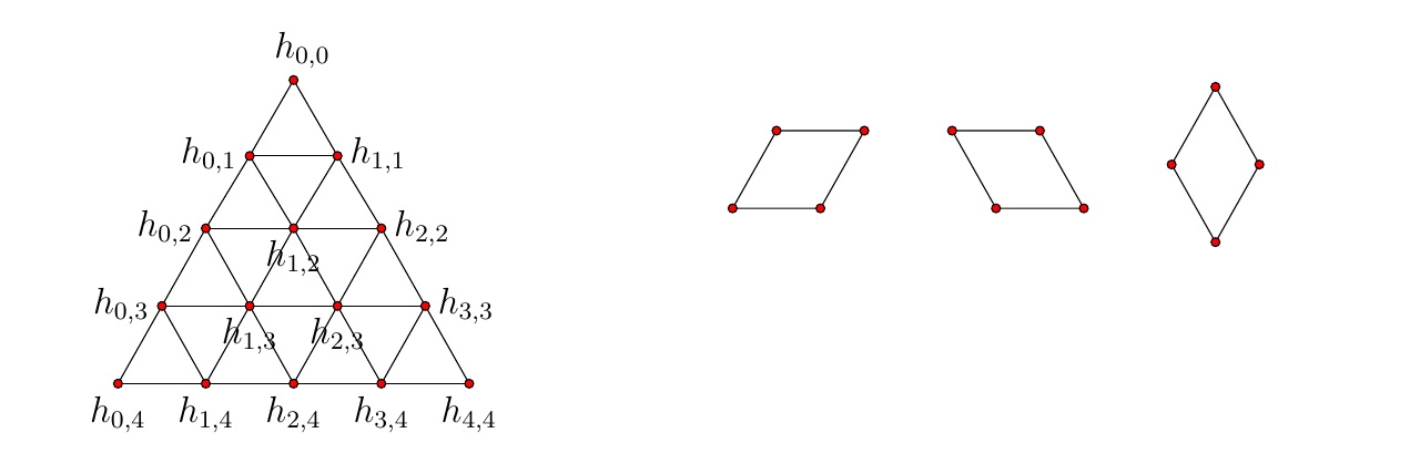
Let \(\lambda = (\lambda_1, \dots, \lambda_k), \mu = (\mu_1, \dots, \mu_k), \nu = (\nu_1, \dots, \nu_k)\) be partitions with at most \(k\) parts such that \(|\nu| = |\lambda| + |\mu|.\) A hive of type \((\nu, \lambda, \mu)\) is a labelling \((h_{i,j})\) of \(\Delta_k\) that satisfies the following hive conditions.
Boundary condition: The labelings on the boundary are determined by \(\lambda, \mu, \nu\) in the following ways. \[\begin{aligned} &h_{0,0} = 0, \ h_{j, j} – h_{j-1, j-1} = \nu_j, \ h_{0,j} – h_{0,j-1} = \lambda_j, &\text{ for } 1 \leq j \leq k.\\ &h_{i,k} – h_{i-1,k} = \mu_i, &\text{ for } 1 \leq i \leq k. \end{aligned}\]
Rhombi condition: For every rhombus, the sum of the labels at obtuse vertices is greater than or equal to the sum of the labels at acute vertices. That is, for \(1 \leq i < j \leq k,\) \[\begin{aligned} h_{i,j} – h_{i,j-1} &\geq h_{i-1, j} – h_{i-1, j-1},\\ h_{i,j} – h_{i-1, j} &\geq h_{i+1, j+1} – h_{i,j+1}, \end{aligned}\] and \[\begin{aligned} h_{i-1, j} – h_{i-1, j-1} &\geq h_{i,j+1} – h_{i,j}. \end{aligned}\]
Let \(H_k(\nu,\lambda,\mu)\) denote the set of all hives of type \((\nu, \lambda, \mu)\). Then the hive conditions (HC1) and (HC2) imply that \(H_k(\nu,\lambda,\mu)\) is a rational polytope in \(\mathbb{R}^{n}\) where \(n = \binom{k+2}{2}\). Hence, we will call \(H_k(\nu,\lambda,\mu)\) the hive polytope of type \((\nu,\lambda,\mu)\). Knutson-Tao [7] and Buch [2] showed that \[c^{\nu}_{\lambda,\mu} = \text{ the number of integer points in } H_k(\nu,\lambda,\mu).\]
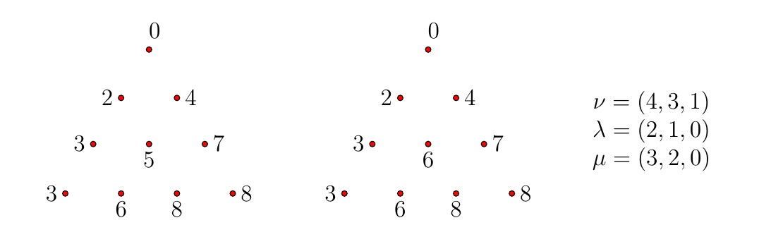
Example 2.2. Let \(k = 3\), \(\nu = (4,3,1), \lambda = (2,1,0),\) and \(\mu = (3,2,0)\), we have that \(c^{\nu}_{\lambda,\mu} = 2\). The two corresponding integer points (integer labels) of \(H_{3}(\nu, \lambda, \mu)\) are shown in Figure 2.
For fixed partitions \(\lambda, \mu, \nu\) with at most \(k\) parts such that \(|\nu| = |\lambda| + |\mu|\), we define the the stretched Littlewood-Richardson coefficient to be the function \(c^{t\nu}_{t\lambda,t\mu}\) for non-negative integer \(t.\) Because \(H_k(t\nu,t\lambda,\\ t\mu) = tH_k(\nu,\lambda,\mu)\), we have that \[c^{t\nu}_{t\lambda,t\mu} = i(H_k(\nu,\lambda,\mu),t).\]
Examples provided in [6] indicate that \(H_k(\nu,\lambda,\mu)\) is in general not an integral polytope. Thus, by Ehrhart theory (Theorem 2.1), \(c^{t\nu}_{t\lambda,t\mu}\) is a quasi-polynomial in \(t\). We will show that \(c^{t\nu}_{t\lambda,t\mu}\) is indeed a polynomial in \(t\) even though the corresponding hive polytope \(H_k(\nu,\lambda,\mu)\) is not integral.
We will show the polynomiality of \(c^{t\nu}_{t\lambda,t\mu}\) by using Steinberg’s formula as derived in [11] by Rassart and the chamber complex of the Kostant partition function. To this end, we state the related notations and results for later reference.
Let \(e_1, \dots, e_k\) be the standard basis vectors in \(\mathbb{R}^k\), and let \(\Delta_+ = \{e_i – e_j: 1 \leq i < j \leq k\}\) be the set of positive roots of the root system of type \(A_{k-1}.\) We define \(M\) to be the matrix whose columns consist of the elements of \(\Delta_+\). The Kostant partition function for the root system of type \(A_{k-1}\) is the function \(K: \mathbb{Z}^k \longrightarrow \mathbb{Z}_{\geq 0}\) defined by \[K(v) = \Big\vert\left\{b \in \mathbb{Z}_{\geq 0}^{\binom{k}{2}}\,|\, Mb = v\right\}\Big\vert.\]
That is, \(K(v)\) equals the number of ways to write \(v\) as nonnegative integer linear combinations of the positive roots in \(\Delta_+\).
An important property of the matrix \(M\), when written in the basis of simple roots \(\{e_i – e_{i+1}\,|\, i = 1, \dots, k-1\}\), is that it is totally unimodular, i.e. the determinant of every square submatrix equals \(-1, 0,\) or \(1.\) Indeed, it was shown in [13] that a matrix \(A\) is totally unimodular if every column of \(A\) only consists of 0’s and 1’s in a way that the 1’s come in a consecutive block. Let \[\mathrm{cone}(\Delta_+) = \left\{\sum \lambda_v v\,|\, v \in \Delta_+, \lambda_v \geq 0\right\},\] be the cone spanned by the vectors in \(\Delta_+.\) The chamber complex is the polyhedral subdivision of \(\mathrm{cone}(\Delta_+)\) that is obtained from the common refinement of cones \(\mathrm{cone}(B)\) where \(B\) are the maximum linearly independent subsets of \(\Delta_+\). A maximum cell (a cone of maximum dimension) \(\cal C\) in the chamber complex is called a chamber. Since \(M\) is totally unimodular, the behavior of \(K(v)\) is given by the following lemma as a special case of [16, Theorem 1] due to Sturmfels.
Lemma 2.3. Let \(\cal C\) be a chamber in the chamber complex of \(\mathrm{cone}(\Delta_+)\). Then the Kostant partition function \(K(v)\) is a polynomial in \(v = (v_1, \dots, v_k)\) on \(\cal C\) of degree at most \(\binom{k-1}{2}\).
Steinberg’s formula [15] expresses the tensor product of two irreducible representations of semisimple Lie algebras as the direct sum of other irreducible representations. When restricting the formula to \(\mathrm{SL}_k\mathbb{C}\), we obtain the following version of Steinberg’s formula for computing \(c^{\nu}_{\lambda,\mu}\).
Theorem 2.4. Let \(\mu, \lambda, \nu\) be partitions with at most \(k\) part such that \(|\nu| = |\lambda| + |\mu|.\) Then \[c^{\nu}_{\lambda,\mu} = \sum_{\sigma,\tau \in \cal S_k}(-1)^{\mathrm{inv}(\sigma\tau)}K(\sigma(\lambda +\delta) + \tau(\mu + \delta) – (\nu + 2\delta)),\] where \(\mathrm{inv}(\psi)\) is the number of inversions of the permutation \(\psi\) and \[\delta = \frac{1}{2}\sum_{1 \leq i < j \leq k}(e_i – e_j) = \frac{1}{2}(k-1, k-3, \dots, -(k-3), -(k-1)),\] is the Weyl vector for type \(A_{k-1}.\)
Details of the derivation can be found in [11].
We are now ready to prove Theorem 1.1.
Proof of Theorem 1.1. The hive conditions imply that \(c^{t\nu}_{t\lambda, t\mu}\) is a quasi-polynomial in \(t.\) To see that \(c^{t\nu}_{t\lambda, t\mu}\) is in fact a polynomial in \(t\), it suffices to show that there exists an integer \(N\) such that \(c^{t\nu}_{t\lambda, t\mu}\) is a polynomial in \(t\) for \(t \geq N.\)
For \(\sigma, \tau \in \cal S_k\), let \[\begin{aligned} r^{\lambda,\mu,\nu}_{\sigma,\tau}(t) &:= \sigma(t\lambda + \delta) + \tau(t\mu+\delta) – (t\nu +2\delta)= t(\sigma(\lambda) +\tau(\mu) – \nu) + \sigma(\delta)+\tau(\delta)-2\delta. \end{aligned}\]
Then \(r^{\lambda,\mu,\nu}_{\sigma,\tau}(t)\) is a ray (when allowing \(t\) to be non-negative real number) emanating from \(\sigma(\delta)+\tau(\delta)-2\delta\) in the direction of \(\sigma(\lambda) +\tau(\mu) – \nu\).
By Steinberg’s formula, \[c^{t\nu}_{t\lambda, t\mu} = \sum_{\sigma, \tau \in \cal S_k}(-1)^{\mathrm{inv}(\sigma\tau)}K\left(r^{\lambda,\mu,\nu}_{\sigma,\tau}(t)\right).\]
Lemma 2.3 states that \(K(v)\) is a polynomial in \(v\) when \(v\) stays in one particular cone (chamber) of the chamber complex of \(\mathrm{cone}(\Delta_+)\). Because there are only finitely many cones in the chamber complex, we have that for every pair \(\sigma, \tau \in \cal S_k\) there exists an integer \(N^{\lambda,\mu,\nu}_{\sigma,\tau}\) such that exactly one of the following happens:
(1) The ray \(r^{\lambda,\mu,\nu}_{\sigma,\tau}(t)\) lies in one particular cone of the chamber complex for all \(t \geq N^{\lambda,\mu,\nu}_{\sigma,\tau},\)
(2) The ray \(r^{\lambda,\mu,\nu}_{\sigma,\tau}(t)\) lies outside \(\mathrm{cone}(\Delta_+)\) for all \(t \geq N^{\lambda,\mu,\nu}_{\sigma,\tau}.\)
If (1) is satisfied, then \(K(r^{\lambda,\mu,\nu}_{\sigma,\tau}(t))\) is a polynomial in \(t\) for \(t \geq N^{\lambda,\mu,\nu}_{\sigma,\tau}\). If (2) is satisfied, then \(K(r^{\lambda,\mu,\nu}_{\sigma,\tau}(t))\) is the zero polynomial for \(t \geq N^{\lambda,\mu,\nu}_{\sigma,\tau}.\) In either case, \(K(r^{\lambda,\mu,\nu}_{\sigma,\tau}(t))\) is a polynomial in \(t\) for \(t \geq N^{\lambda,\mu,\nu}_{\sigma,\tau}\). Now let \[N = \max_{\sigma, \tau \in \cal S_k}\left\{ N^{\lambda,\mu,\nu}_{\sigma,\tau}\right\}.\]
Then Steinberg’s formula implies that \(c^{t\nu}_{t\lambda, t\mu}\) is a polynomial in \(t\) for \(t \geq N.\) Therefore, \(c^{t\nu}_{t\lambda, t\mu}\) is a polynomial in \(t\).
By Lemma 2.3, each polynomial piece of \(K(v)\) has degree at most \(\binom{k-1}{2}\). Thus, for every \(\sigma, \tau\), we have that \(K\left(r^{\lambda,\mu,\nu}_{\sigma,\tau}(t)\right)\) is a polynomial in \(t\) of degree at most \(\binom{k-1}{2}\) for \(t \geq N^{\lambda,\mu,\nu}_{\sigma,\tau}.\) Hence, \(c^{t\nu}_{t\lambda, t\mu}\) is a polynomial in \(t\) of degree at most \(\binom{k-1}{2}\). ◻
In the proof of Theorem 1.1, we showed that every \(K(r^{\lambda,\mu,\nu}_{\sigma,\tau}(t))\) is eventually either the zero polynomial or a non-zero polynomial in \(t\). Proposition 3.2 gives a characterization of those \(K(r^{\lambda,\mu,\nu}_{\sigma,\tau}(t))\) that eventually become nonzero polynomials. The proof uses the following characterization of nonzero \(K(v)\).
Lemma 3.1. Let \(v = (v_1, \dots, v_k)\) be a vector in \(\mathbb{Z}^k\) with \(v_1 + \cdots + v_k = 0\). Then \(K(v)\) is nonzero if and only if \(v_1 + \cdots + v_i \geq 0\) for all \(i = 1, \dots, k\).
Proof. Let \(M^*\) be the matrix \(M\) written using the simple roots \(e_1 – e_{2}, \dots, e_{k-1} – e_k\) as a basis. Then, the entries of \(M^*\) are only \(0\) and \(1\). Moreover, because the simple roots themselves are columns of \(M\), we have that the identity matrix is a submatrix of \(M^*\). Similarly, let \(v^*\) be the vector \(v\) written using the simple roots as a basis. Then, \(v^* = (v_1, v_1+v_2, \dots, v_1 + \cdots v_{k-1})\). The desired result is obtained by observing that \(K(v) = \left\vert\left\{b \in \mathbb{Z}_{\geq 0}^{\binom{k}{2}}\,|\, M^*b = v^*\right\}\right\vert.\) ◻
Proposition 3.2. Let \(\mu, \lambda, \nu\) be partitions with at most \(k\) part such that \(|\nu| = |\lambda| + |\mu|.\) For \(\sigma, \tau \in \cal S_k,\) let \(r^{\lambda,\mu,\nu}_{\sigma,\tau}(t) = t\beta + \gamma\) where \(\beta = \sigma(\lambda) +\tau(\mu) – \nu\) and \(\gamma = \sigma(\delta)+\tau(\mu)-2\delta.\) Then there exists an integer \(N^{\lambda,\mu,\nu}_{\sigma,\tau}\) such that \(K(r^{\lambda,\mu,\nu}_{\sigma,\tau}(t))\) is a non-zero polynomial in \(t\) for \(t \geq N^{\lambda,\mu,\nu}_{\sigma,\tau}\) if and only if for all \(i = 1, \dots, k\) we have that
(1) \(\beta_1 + \beta_2 + \cdots + \beta_i\) is positive, or
(2) \(\beta_1 + \beta_2 + \cdots + \beta_i\) is zero and \(\gamma_1 + \gamma_2 + \cdots + \gamma_i\) is non-negative.
Proof. Let \(r^{\lambda,\mu,\nu}_{\sigma,\tau}(t) = (r_1(t), \dots, r_k(t))\). Then \(r_i(t) = t\beta_i + \gamma_i\). In the proof of Theorem 1.1, we showed that there exists a positive integer \(N^{\lambda,\mu,\nu}_{\sigma,\tau}\) such that \(K(r^{\lambda,\mu,\nu}_{\sigma,\tau}(t))\) is a polynomial in \(t\) for \(t \geq N^{\lambda,\mu,\nu}_{\sigma,\tau}.\) For every \(i = 1, \dots, k\), the partial sum \(r_1(t) + \cdots + r_i(t)\) is non-negative for all \(t \geq N^{\lambda,\mu,\nu}_{\sigma,\tau}\) precisely when one of the two conditions meets for all \(i = 1, \dots, k\). Thus, by Lemma 3.1, \(K(r^{\lambda,\mu,\nu}_{\sigma,\tau}(t))\) is a non-zero polynomial for \(t \geq N^{\lambda,\mu,\nu}_{\sigma,\tau}.\) ◻
I am grateful to Fu Liu. Her careful review and thoughtful comments significantly improved the exposition of this paper. I also would like to thank UC Davis’s College of Letter and Science for providing the Dean’s Summer Graduate Fellowship to support me during the summer of 2022.