
Degree-based indices have grown since topological invariants were first developed and used in Chemical Graph Theory (CGT). Nowadays, research on chemical applications and mathematical properties of degree-based topological invariants are significantly active, see [4, 13]. The reason behind the sudden increase in the introduction of these indices could be attributed to their straightforward definitions, computationally easy techniques and unexpectedly good performance in predicting the physico-chemical properties of molecules. The study of degree-based topological indices is applied mathematically to irregularity measures and metrics of graph branching [1].
Throughout this article, we consider a simple, connected and undirected graph \(\varUpsilon=(V(\varUpsilon),E(\varUpsilon))\), with \(V(\varUpsilon)\) and \(E(\varUpsilon)\) as its vertex and edge set, respectively. The degree \(\Im_{u}\) of a vertex \(u\in V(\varUpsilon)\) is the total number of edges associated with that vertex. Also, \(|V(\varUpsilon)|=n\) and \(|E(\varUpsilon)|=m\) are the order and size of the graph, respectively. We use \(\delta\) and \(\Delta\) to denote the minimum degree and maximum degree of the graph \(\varUpsilon\), respectively [41].
Since when the idea of topological molecular descriptors is employed, several notable degree-based topological descriptors have been introduced. Below we state some standard topological descriptors which will be utilized in the rest of this article.
One of the oldest degree-dependent topological indices is the Zagreb indices [19]. Gutman and Trinajstic introduced them in 1972 and defined them as follows: \[\label{Def:M1} M_{1}(\varUpsilon)= \sum_{uv\in E(\varUpsilon)}(\Im_{u}+\Im_{v}),\tag{1}\] and \[\label{Def:M2} M_{2}(\varUpsilon) = \sum_{uv\in E(\varUpsilon)}\Im_{u}\cdot \Im_{v}.\tag{2}\]
Despite their age, they are appropriate and significant even today and several publications on Zagreb indices are appearing [14, 20, 42].
The forgotten index was seen in the same article as the Zagreb indices [19], but it was sitting in the shadow for almost 40 years. Later, B. Furtula and I. Gutman reintroduced it in [16] and defined as follows:
\[\label{Def:F} F(\varUpsilon)= \sum_{uv\in E(\varUpsilon)}(\Im^{2}_{u}+\Im^{2}_{v}).\tag{3}\]
Recently in [21, 32], the forgotten topological index of a graph and its some new inequalities are investigated.
Randić index [35] is a widely employed well-known degree-based topological index. It is defined as follows: \[\label{Def:R} R(\varUpsilon)=\sum_{uv\in E(\varUpsilon)}\frac{1}{\sqrt{\Im_{u}\cdot \Im_{v}}}.\tag{4}\]
For more than 40 years, the Randić index has been studied, resulting in hundreds of publications and numerous books [3,5, 31,33]. Several improvements to this index have been put forward in order to improve its predictive potential [33]. One of such improvements is the reciprocal Randić index which is defined as \[\label{Def:RR} \textit{RR}(\varUpsilon)=\sum_{uv\in E(\varUpsilon)}\sqrt{\Im_{u}\cdot \Im_{v}}.\tag{5}\]
In 2013, the idea of the first and second hyper-Zagreb indices are proposed in [37] and they are defined as follows: \[\label{Def:HM1} \textit{HM}_{1}(\varUpsilon)= \sum_{uv\in E(\varUpsilon)}(\Im_{u}+\Im_{v})^2,\tag{6}\] and \[\label{Def:HM2} \textit{HM}_{2}(\varUpsilon) = \sum_{uv\in E(\varUpsilon)}(\Im_{u}\cdot \Im_{v})^2.\tag{7}\]
Later, these indices were also studied for several classes of graphs in [6, 17].
More than one decades ago, the idea of symmetric division deg index of a graph \(\varUpsilon\) is proposed in [38]. We denote it as \(\textit{SDD}(\varUpsilon)\) and it is defined as \[\label{Def:SDD} \textit{SDD}(\varUpsilon)=\sum_{uv\in E(\varUpsilon)}\bigg(\frac{\Im_{u}}{\Im_{v}}+\frac{\Im_{v}}{\Im_{u}}\bigg).\tag{8}\]
Moreover, it has just lately gained a lot of interest because of its some reasonable predictive capability [2,15].
Recently, I. Gutman proposed three novel topological indices one of them was Sombor index [18], and defined as follows: \[\label{Def:SO} \textit{SO}(\varUpsilon)=\sum_{uv\in E(\varUpsilon)}\sqrt{\Im^{2}_{u}+\Im^{2}_{v}}.\tag{9}\]
Geometrically, the Sombor index is a measure of the distance of the point \((\Im_u,\Im_v)\) from the origin in the \(2D\) Cartesian coordinate system. A new method to compute the different ombor-type indices via -polynomial was proposed in [29].
Inspired by the work on Sombor index, V.R. Kulli proposed Nirmala index [23] of the graph \(\varUpsilon\) and defined as follows: \[\label{Def:N} N(\varUpsilon)=\sum_{uv\in E(\varUpsilon)}\sqrt{\Im_{u}+\Im_{v}}.\tag{10}\]
Further, the first inverse Nirmala index (denoted as \(\textit{IN}_1(\varUpsilon)\)) and second inverse Nirmala index (denoted as \(\textit{IN}_2(\varUpsilon)\)) of a molecular graph \(\varUpsilon\) are established by Kulli et al. [25] in \(2021\) which are defined as follows: \[\label{Def:IN1} \textit{IN}_1(\varUpsilon)=\sum_{uv \in E(\varUpsilon)} \sqrt{\frac{1}{\Im_{u}}+\frac{1}{\Im_{v}}}=\sum_{uv \in E(\varUpsilon)} \sqrt{\frac{\Im_{u}+\Im_{v}}{\Im_{u}\Im_{v}}},\tag{11}\]
\[\label{Def:IN2} \textit{IN}_2(\varUpsilon)=\sum_{uv \in E(\varUpsilon)} \frac{1}{\sqrt{\frac{1}{\Im_{u}}+\frac{1}{\Im_{v}}}}=\sum_{uv \in E(\varUpsilon)} \sqrt{\frac{\Im_{u}\Im_{v}}{\Im_{u}+\Im_{v}}}.\tag{12}\]
Lately, the derivation formulas of Nirmala indices and its generalized version ((\(a,b\))-Nirmala index) based on M-polynomials were suggested in [10,11]. Comparative study between irmala and ombor indices based on their applicability, degeneracy and smoothness was presented in [28,26]. The ordhaus-addum-type inequalities for the irmala Indices were obtained in the article [30].
In the year 2022, V.R. Kulli proposed two novel topological indices based on the geometric and quadratic mean of degrees of end vertices of an edge \(uv\in E(\varUpsilon)\). They are named as geometric-quadratic (GQ) and quadratic-geometric (QG) indices [24]. The mathematical definitions of the GQ and QG indices are:
\[\label{Def:GQ} \textit{GQ}(\varUpsilon)=\sum_{uv\in E(\varUpsilon)}\frac{\sqrt{2\Im_{u}\Im_{v}}}{\sqrt{\Im^{2}_{u}+\Im^{2}_{v}}},\tag{13}\] and \[\label{Def:QG} \textit{QG}(\varUpsilon)=\sum_{uv\in E(\varUpsilon)}\frac{\sqrt{\Im^{2}_{u}+\Im^{2}_{v}}}{\sqrt{2\Im_{u}\Im_{v}}}.\tag{14}\]
The computation of the GQ and QG indices for some standard graphs and jagged-rectangle benzenoid system was reported in [24,8]. The GQ and QG indices-based entropy measures of some silicon carbide networks were computed in [9].
Apart from the above mathematical developments on GQ and QG indices, one can find the evidence of usability of the indices in the article [12].
In this article, the authors performed the Quantitative Structure-Property Relationship (QSPR) analysis to predict the physico-chemical properties of certain well-known COVID-19 drugs, where the GQ and QG indices have shown a good correlation with some of the physico-chemical properties of the drugs. The cubic regression models corresponding to the indices with the squared correlation coefficients \(0.9910\) and \(0.9872\), respectively (determined in Table 8 of [12]), depict that the indices predict the mass (M) of the drugs significantly. For more details, readers can see Tables 8 and 9, Figure 18(b) and point number (vi) in the conclusion section of the recently published article [12]. Moreover, very recently, the authors of [27] examined the newly defined GQ–QG indices’ chemical applicability and compare their prediction power, degeneracy, and structural sensitivity to those of existing notable degree-based topological indices.
| \(\mbox{ Benzenoid hydrocarbons~$\downarrow$}\) | Topological index | Physico-chemical properties | |||||
|---|---|---|---|---|---|---|---|
| \(GQ\) | \(QG\) | BP | DHFORM | MW | \(\log P\) | \(E_\pi\) | |
| Benzene | \(6.0000\) | \(6.0000\) | \(80.1000\) | \(75.2000\) | \(78.1100\) | \(8.0000\) | \(2.1300\) |
| Naphthalene | \(10.8431\) | \(11.1633\) | \(218.0000\) | \(141.0000\) | \(128.1710\) | \(13.6790\) | \(3.3000\) |
| Phenanthrene | \(15.7646\) | \(16.2450\) | \(338.0000\) | \(202.7000\) | \(178.2340\) | \(19.5000\) | \(4.4600\) |
| Anthracene | \(15.6862\) | \(16.3267\) | \(340.0000\) | \(222.6000\) | \(178.2340\) | \(19.3090\) | \(4.4500\) |
| Chrysene | \(20.6862\) | \(21.3267\) | \(431.0000\) | \(271.1000\) | \(228.2880\) | \(25.1890\) | \(5.8100\) |
| Benzo[a]anthracene | \(20.6077\) | \(21.4083\) | \(425.0000\) | \(277.1000\) | \(228.2880\) | \(25.0990\) | \(5.7600\) |
| Triphenylene | \(20.7646\) | \(21.2450\) | \(429.0000\) | \(275.1000\) | \(228.2880\) | \(25.3010\) | \(5.4900\) |
| Tetracene | \(20.5292\) | \(21.4899\) | \(440.0000\) | \(310.5000\) | \(228.2880\) | \(25.2010\) | \(5.7600\) |
| Benzo[a]pyrene | \(23.6077\) | \(24.4083\) | \(496.0000\) | \(296.0000\) | \(252.3000\) | \(28.1990\) | \(6.1300\) |
| Benzo[e]pyrene | \(23.6862\) | \(24.3267\) | \(493.0000\) | \(289.9000\) | \(252.3160\) | \(28.2990\) | \(6.4400\) |
| Perylene | \(23.6862\) | \(24.3267\) | \(497.0000\) | \(319.2000\) | \(252.3000\) | \(28.2390\) | \(6.250\) |
| Anthanthrene | \(26.5292\) | \(27.4899\) | \(547.0000\) | \(323.0000\) | \(276.3310\) | \(31.1990\) | \(7.0400\) |
| Benzo[ghi]perylene | \(26.6077\) | \(27.4083\) | \(542.0000\) | \(301.2000\) | \(276.3310\) | \(31.3980\) | \(6.6300\) |
| Dibenzo[a,c]anthracene | \(25.6077\) | \(26.4083\) | \(535.0000\) | \(348.0000\) | \(278.3310\) | \(30.8990\) | \(6.0200\) |
| Dibenzo[a,h]anthracene | \(25.5292\) | \(26.4899\) | \(535.0000\) | \(335.0000\) | \(278.3470\) | \(30.7960\) | \(6.7500\) |
| Dibenzo[a,j]anthracene | \(25.5292\) | \(26.4899\) | \(531.0000\) | \(336.3000\) | \(281.3000\) | \(30.7950\) | \(6.5400\) |
| Picene | \(25.6077\) | \(26.4083\) | \(519.0000\) | \(336.9000\) | \(278.3000\) | \(30.8910\) | \(7.1100\) |
| Coronene | \(29.5292\) | \(30.4899\) | \(590.0000\) | \(296.7000\) | \(300.4000\) | \(34.6010\) | \(7.6400\) |
| Dibenzo(a,h)pyrene | \(28.5292\) | \(29.4899\) | \(59.00006\) | \(375.6000\) | \(302.4000\) | \(33.8550\) | \(7.2800\) |
| Dibenzo(a,i)pyrene | \(28.5292\) | \(29.4899\) | \(594.0000\) | \(366.0000\) | \(302.4000\) | \(33.8790\) | \(7.2800\) |
| Dibenzo(a,l)pyrene | \(28.6077\) | \(29.4083\) | \(595.0000\) | \(393.3000\) | \(302.4000\) | \(34.0090\) | \(7.2800\) |
| Pyrene | \(18.6862\) | \(19.3267\) | \(393.0000\) | \(221.3000\) | \(202.2560\) | \(22.4950\) | \(4.8800\) |
Hence, the study of the mathematical properties and bounds of the GQ and QG indices is worthy of investigation in the field of chemical graph theory.
The rest of the manuscript is built as follows. The chemical applicability of the considered GQ and QG indices is investigated over the physico-chemical properties of 22 benzenoid hydrocarbons in Section 2. In Section 3, some tight upper and lower bounds for the GQ and QG indices in terms of size, degree sequence of a graph and the above-mentioned degree-based topological indices are established. Section 4 is reserved for the conclusion.
The novel topological indices should correlate well with one of the physico-chemical properties of a molecular compound. The ability to discriminate between isomers, predictive power and smoothness of the GQ and QG indices have been investigated in article [27]. Here, we focus our attention to test the chemical applicability of the concerned indices over the physico-chemical properties of \(22\) benzenoid hydrocarbons. Benzenoid hydrocarbons are a specific type of organic compound with a condensed polycyclic structure made up only of hexagonal rings. It has been utilized by numerous researchers to evaluate the strength and quality of different molecular descriptors and structural invariants for QSPR/QSAR analysis [34]. These chemical graphs have notable variance, shape, non-polarity, and branching because of the diversity of their structures. Many researchers have conducted a variety of studies on benzenoid hydrocarbons, see [22, 7, 36,39]. The physico-chemical properties such as boiling point (BP), standard heat of formation (DHFORM), molecular weight (MW), \(log~P\) and \(\pi\)-electron energy (\(E_{\pi}\)) of benzenoid hydrocarbons are comprised from the article [7, 39]. These properties together with the computed values of GQ–QG indices of benzenoid hydrocarbons are cataloged in Table 1 to perform the linear regression analysis.
\[\label{Eqn:LRM} P=p_1\times TI +p_2,\tag{15}\] is performed for regression analysis. In Eq. (15), \(P\) denotes the physico-chemical property, \(\textit{TI}\) symbolizes the topological index and \(p_{i}\) where \(i=1,2\) represent the fitting coefficients.
The linear regression models are performed using MATLAB R2019a software and fitting coefficients \(p_1\) and \(p_2\) are taken with \(95\%\) confidence bounds. The statistical parameters obtained from linear regression analysis are \(R^2\), \(Adj\)–\(R^2\), root mean square error (RMSE) and sum of square error (SSE).
The squared of correlation-coefficient (\(R^2\)) closer to \(1\) and RMSE near to \(0\) represent the goodness of a linear regression model. The linear regression models for GQ and QG indices with different physico-chemical properties of benzenoid hydrocarbons are detailed below.
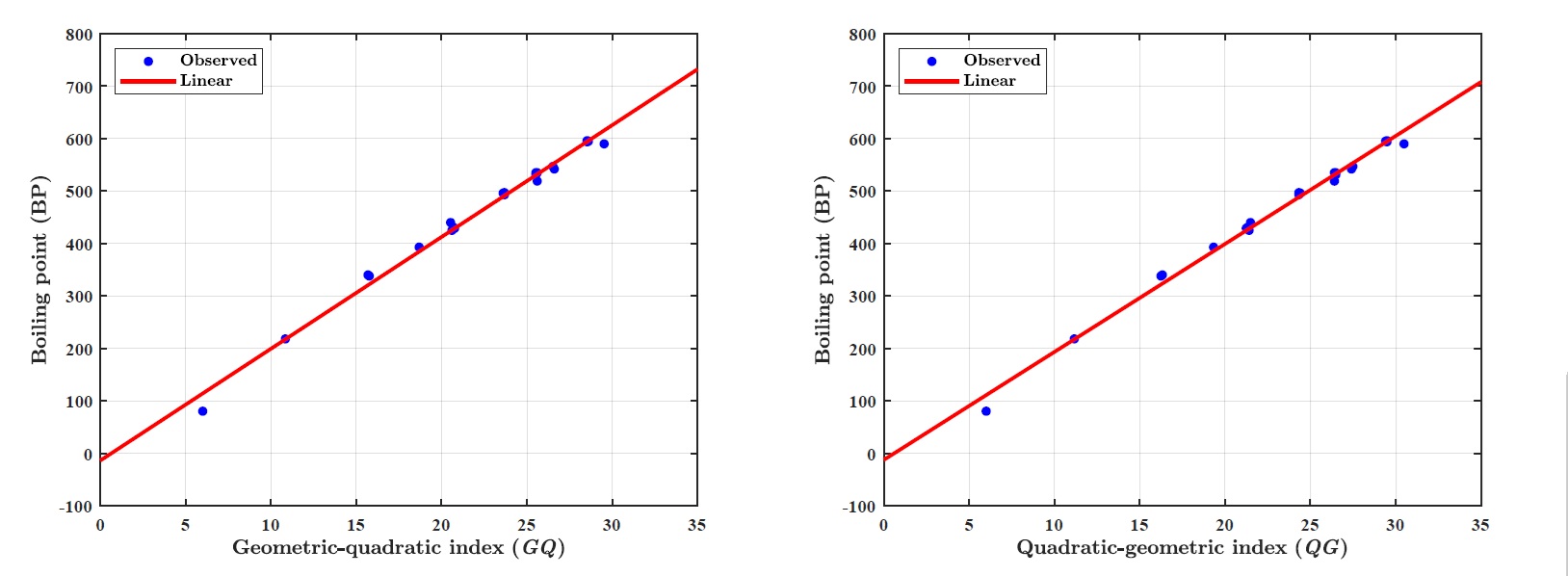
(i) Boiling point (BP):
LRM for GQ index: \(BP = p_1\times\textit{GQ} + p_2\), where coefficients (with \(95\%\) confidence bounds) \(p_1 =21.3200 (20.3600, 22.2800)~\text{and}~p_2 =-13.9000(-36.0600, 8.2670).\)
Goodness of fit:\(R^2=0.9908,~\textit{Adj-}R^2=0.9903,~\textit{SSE}=3227~\text{and}~\textit{RMSE}=12.7000\)
LRM for QG index: \(BP= p_1\times \textit{QG} + p_2\), where coefficients (with \(95\%\) confidence bounds) \(p_1 = 20.5900 (19.7300, 21.4500),~ p_2 = -12.6900 (-33.1700, 7.7920)\).
Goodness of fit:\(~R^2=0.9921,~\textit{Adj-}R^=0.9917~ \textit{SSE}=2772~\text{and}~\textit{RMSE}=11.7700.\)
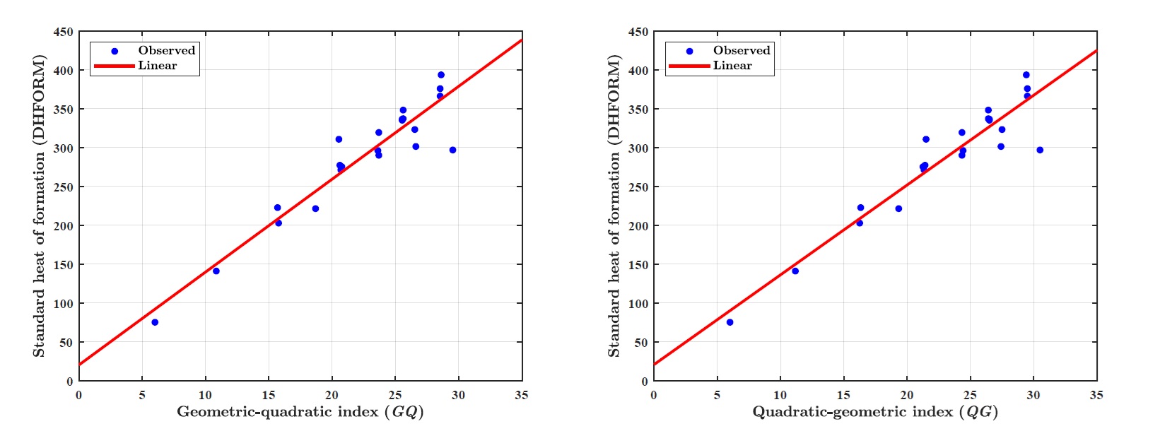
(ii) Standard enthalpy of formation (DHFORM):
LRM for GQ index: \(DHFORM = p_1\times \textit{GQ} + p_2\), where coefficients (with \(95\%\) confidence bounds) \(p_1 = 11.9400 (10.0000, 13.8800) p_2 = 20.3600 (-24.4500, 65.1700).\)
Goodness of fit: \(R^2 =0.8917,~ \textit{Adj-}R^2=0.8863,~ \textit{SSE} = 1.319e+04~ \text{and}~\textit{RMSE}=25.6800.\)
LRM for QG index: \(DHFORM = p_1\times \textit{QG} + p_2\), where coefficients (with \(95\%\) confidence bounds): \(p1 = 11.5500 (9.6980, 13.4000),~ p2 = 20.7900 (-23.2900, 64.8700).\)
Goodness of fit: \(R^2=0.8946,~ \textit{Adj-}R^2=0.8893,~ \textit{SSE}=1.284e+04~\text{and}~ \textit{RMSE}=25.3400.\)
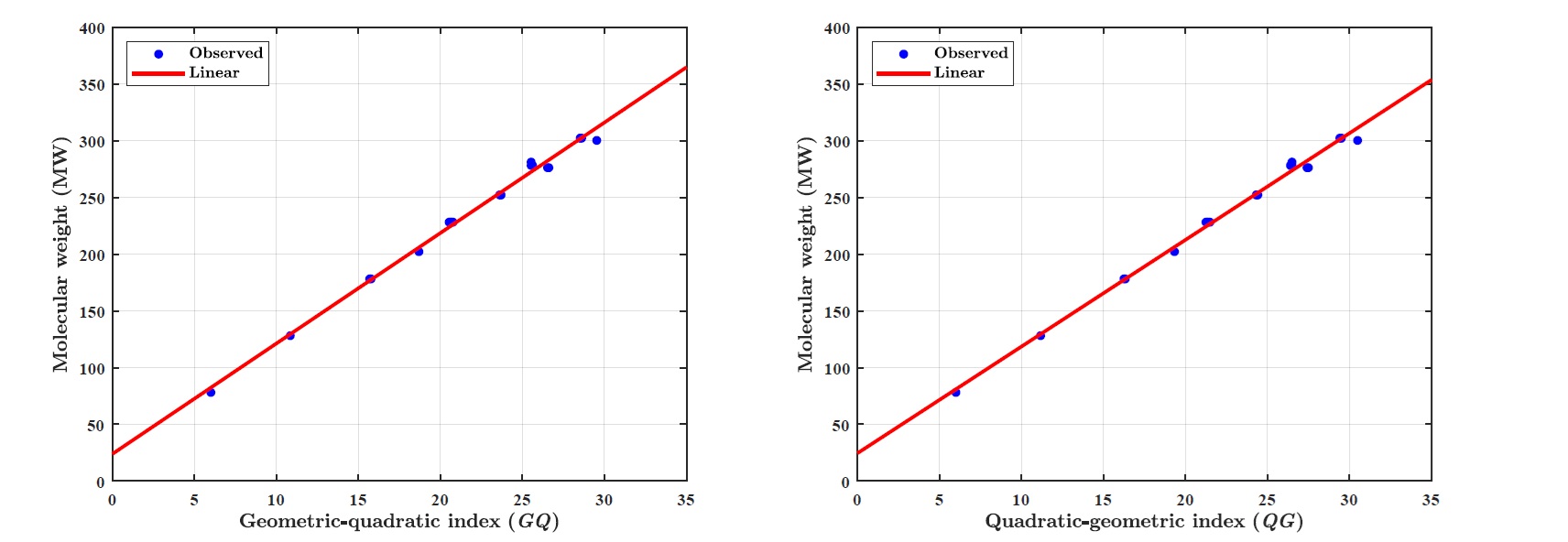
(iii) Molecular weight (MW):
LRM for molecular weight (MW): \(MW = p_1\times \textit{GQ} + p_2\), where coefficients (with \(95\%\) confidence bounds): \(p_1 = 9.7450 (9.3830, 10.1100),~ p_2 = 23.8700 (15.5000, 32.2400).\)
Goodness of fit: \(R^2=0.9937,~ \textit{Adj-}R=0.9934,~ \textit{SSE}=460~\text{and}~ \textit{RMSE}=4.7960.\)
LRM for molecular weight (MW): \(MW = p_1\times \textit{QG}+ p_2\), where coefficients (with \(95\%\) confidence bounds): \(p_1 = 9.4110 (9.0820, 9.740),~p_2 = 24.4900 (16.6400, 32.3400).\)
Goodness of fit: \(R^2=0.9944,~ \textit{Adj-}R^2=0.9941,~ \textit{SSE}=407.1000~\text{and}~ \textit{RMSE}=4.5120.\)
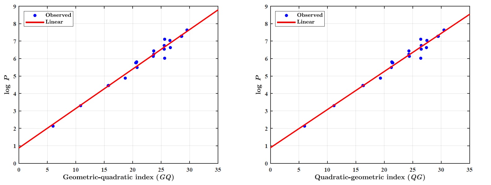
(iv)
LRM for GQ index: \(log~P= p_1\times GQ+ p_2\), where coefficients (with \(95\%\) confidence bounds): \(p_1 =0.2262 (0.2090, 0.2435),~p_2 =0.8776 (0.4793, 1.2760).\)
Goodness of fit: \(R^2=0.9740,~ \textit{Adj-}R^2=0.9727,~ \textit{SSE}=1.0420~\text{and}~ \textit{RMSE}=0.2282.\)
LRM for QG index: \(log~P= p_1\times QG+ p_2\), where coefficients (with \(95\%\) confidence bounds): \(p_1 =0.2185 (0.2022, 0.2348),~p_2 =0.8908 (0.5024, 1.2790).\)
Goodness of fit: \(R^2=0.9751,~ \textit{Adj-}R^2=0.9739,~ \textit{SSE}=0.9967~\text{and}~ \textit{RMSE}=0.2232.\)
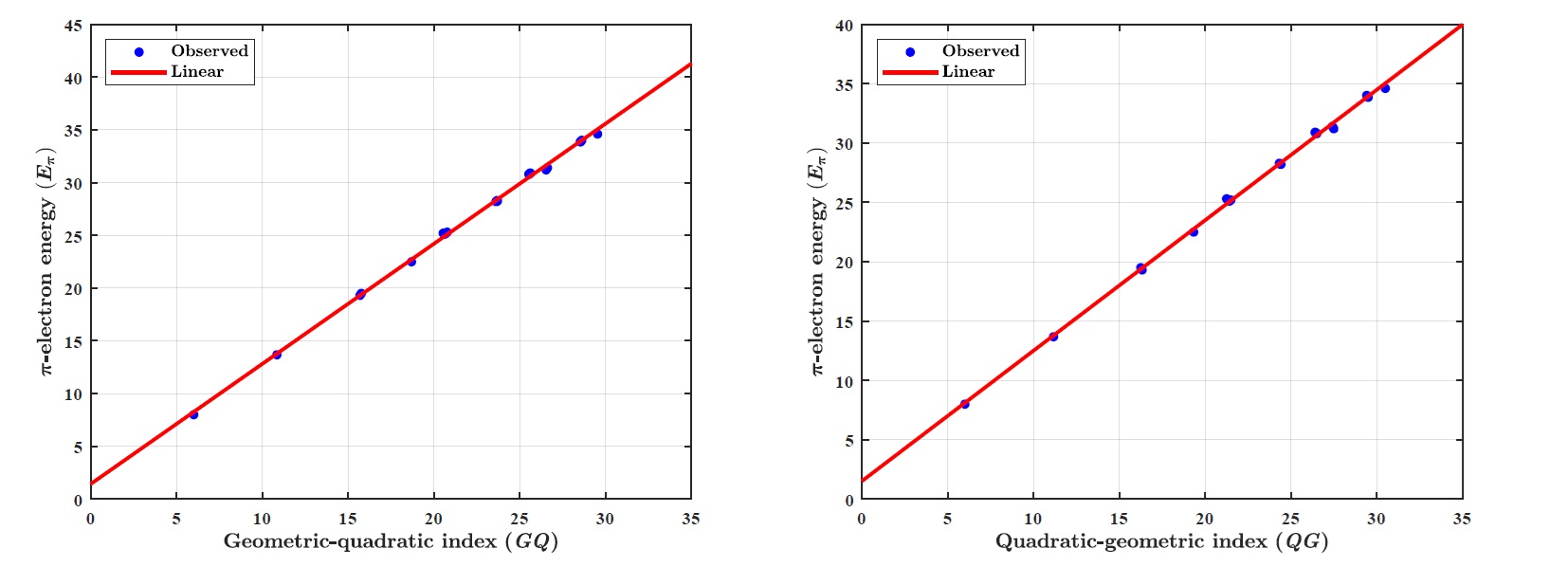
(v) \(\pi\)-electron energy (\(E_{\pi}\)):
LRM for GQ index: \(E_{\pi}= p_1\times GQ+ p_2\), where coefficients (with \(95\%\) confidence bounds): \(p_1 =1.1380 (1.1190, 1.1580),~p_2 =1.4400(0.9862, 1.8930).\)
Goodness of fit: \(R^2=0.9986,~ \textit{Adj-}R^2=0.9986,~ \textit{SSE}=1.3520~\text{and}~ \textit{RMSE}=0.2600.\)
LRM for QG index: \(E_{\pi}= p_1\times QG+ p_2\), where coefficients (with \(95\%\) confidence bounds): \(p_1 =1.0990 (1.0810, 1.1170),~p_2 =1.5200 (1.0820, 1.9580).\)
Goodness of fit: \(R^2=0.9987,~ \textit{Adj-}R^2=0.9987,~ \textit{SSE}=1.2700~\text{and}~ \textit{RMSE}=0.2519.\)
We extract the following observations from the above-performed QSPR models:
(i) GQ and QG indices predict the boiling point (BP) with the \(R^2~0.9908\) and \(0.9921\), respectively.
(ii) GQ and QG indices obtain the square correlation coefficient \(R^2\) \(0.8917\) and \(0.8946\), respectively with the standard heat of formation (DHFORM).
(iii) GQ and QG indices forecast the molecular weight (MW) with the \(R^2~0.9937\) and \(0.9944\), respectively.
(iv) GQ and QG indices report the \(R^2\)-values \(0.9740\) and \(0.9751\), respectively, with \(\log~P\) property of benzenoid hydrocarbons.
(v) GQ and QG indices predict the \(\pi\)-electron energy (\(E_{\pi}\)) with the \(R^2~0.9986\) and \(0.9987\), respectively.
Remark 2.1. Both the GQ and QG indices predict the physico-chemical properties of benzenoid hydrocarbons significantly with the correlation-coefficient \(R>0.9\). However, the QG indices shows the more predictive capability in comparison to the GQ index.
Figure 1 illustrates the linear regression model between the \(\textit{GQ}\)–\(\textit{QG}\) indices and the boiling point (BP) of benzenoid hydrocarbons. Figure 2 demonstrates the regression model between the \(\textit{GQ}\)–\(\textit{QG}\) indices and the standard heat of formation (\(\Delta H_{\text{form}}\)). Figure 3 depicts the relationship between the \(\textit{GQ}\)–\(\textit{QG}\) indices and molecular weight (MW). Figure 4 presents the linear regression plot between the \(\textit{GQ}\)–\(\textit{QG}\) indices and logP values of benzenoid hydrocarbons. Finally, Figure 5 shows the regression analysis between the \(\textit{GQ}\)–\(\textit{QG}\) indices and the \(\pi\)-electron energy (\(\pi\)-E).
Here, we establish some tight upper and lower bounds for the GQ and QG indices of a graph \(\varUpsilon\) in terms of its size, degree sequence and some notable degree-based topological descriptors. Before moving further, let us recall a small relation between GQ and QG indices as stated in Theorem 3.1.
Theorem 3.1. [8] Let \(\varUpsilon\) be a simple, connected and undirected graph. Then we have \[0<GQ(\varUpsilon)\leq QG(\varUpsilon).\]
Here, we discuss the bounds of GQ and QG indices in terms of the size and degree of a graph.
Theorem 3.2. Let \(\varUpsilon\) be a simple, connected and undirected graph with \(m\) edges. Then \[\frac{\delta}{\Delta}m\leq GQ(\varUpsilon)\leq m \leq QG(\varUpsilon)\leq \frac{\Delta}{\delta}m.\]
The equality holds if and only if the graph \(\varUpsilon\) is regular.
Proof. To prove this inequality, we use the definitions of GQ and QG indices and the mathematical relation between the geometric mean and quadratic mean of two numbers.
Let us first consider the upper bound of QG index. From Eq. (14), we have \[\begin{aligned} \label{Eq:QG} \textit{QG}(\varUpsilon)=\sum_{uv\in E(\varUpsilon)}\frac{\sqrt{\Im^{2}_{u}+\Im^{2}_{v}}}{\sqrt{2\Im_{u}\Im_{v}}}\leq \sum_{uv\in E(\varUpsilon)}\frac{\sqrt{{\Delta}^{2}+{\Delta}^{2}}}{\sqrt{2\delta\cdot\delta}}\leq \frac{\Delta}{\delta}m. \end{aligned}\tag{16}\]
In a similar way from Eq. (13), we get the lower bound of GQ index as \[\begin{aligned} \label{Eq:GQ} \textit{GQ}(\varUpsilon)=\sum_{uv\in E(\varUpsilon)}\frac{\sqrt{2\Im_{u}\Im_{v}}}{\sqrt{\Im^{2}_{u}+\Im^{2}_{v}}} \geq \sum_{uv\in E(\varUpsilon)}\frac{\sqrt{2\delta\cdot \delta}}{\sqrt{{\Delta}^{2}+{\Delta}^{2}}}\geq \frac{\delta}{\Delta}m. \end{aligned}\tag{17}\]
Next, using the mathematical relation between geometric and quadratic means of two numbers we have \[\sqrt{\Im_{u}\Im_{v}}\leq \sqrt{\frac{\Im^{2}_{u}+\Im^{2}_{v}}{2}} \implies \frac{\sqrt{\Im_{u}\Im_{v}}}{\sqrt{\frac{\Im^{2}_{u}+\Im^{2}_{v}}{2}}}\leq 1 \leq \frac{\sqrt{\frac{\Im^{2}_{u}+\Im^{2}_{v}}{2}}}{\sqrt{\Im_{u}\Im_{v}}}.\]
Now taking the sum over all edges \(uv\in E(\varUpsilon)\) of graph \(\varUpsilon\), we obtain \[\sum_{uv\in E(\varUpsilon)}\frac{\sqrt{2\Im_{u}\Im_{v}}}{\sqrt{\Im^{2}_{u}+\Im^{2}_{v}}}\leq \sum_{uv\in E(\varUpsilon)}1~\leq \sum_{uv\in E(\varUpsilon)} \frac{\sqrt{\Im^{2}_{u}+\Im^{2}_{v}}}{\sqrt{2\Im_{u}\Im_{v}}} ,\] implies, \[\label{Eq:3_GQ-QG}\textit{GQ}(\varUpsilon)\leq m \leq \textit{QG}(\varUpsilon).\tag{18}\]
Hence, by combining Eq. (16) (17) and (18), we have the required result. ◻
The following corollary is straightaway from the above theorem.
Corollary 3.3. Let us consider a \(r\)-regular graph \(\varUpsilon\) with \(m\) edges. Then we have \[GQ(\varUpsilon)=QG(\varUpsilon)=m.\]
In this part, we discuss the bounds of GQ and QG indices in terms of degree sequence and size of a graph.
Theorem 3.4. Let \(\varUpsilon\) be a simple, connected and undirected graph with size \(m\), order \(n\) and degree sequence \(\{\Im_{1},\Im_{2},\ldots ,\Im_{n}\},\) where \(\Im_{1}\geq \Im_{2}\geq \cdots \geq \Im_{n}\). If it has \(p\) number of vertices of degree \(\Im_{n}\), and \(q\) number of edges in the subgraph \(\varGamma\) induced by \(p\) vertices, then
(i) \[\begin{aligned} q+(p\Im_{n}-2q)&\frac{\sqrt{2\Im_{n}\Im_{n-p}}}{\sqrt{\Im^{2}_{n}+\Im^{2}_{1}}}+(m-p\Im_{n}+q)\frac{\Im_{n-p}}{\Im_{1}}\\ &\leq GQ(\varUpsilon) \leq q+(p\Im_{n}-2q)\frac{\sqrt{2\Im_{n}\Im_{1}}}{\sqrt{\Im^{2}_{n}+\Im^{2}_{n-p}}}+(m-p\Im_{n}+q)\frac{\Im_{1}}{\Im_{n-p}}. \end{aligned}\]
(ii) \[\begin{aligned} q+(p\Im_{n}-2q)&\frac{\sqrt{\Im^{2}_{n}+\Im^{2}_{n-p}}}{\sqrt{2\Im_{n}\Im_{1}}}+(m-p\Im_{n}+q)\frac{\Im_{n-p}}{\Im_{1}}\leq QG(\varUpsilon)\\ & \leq q+(p\Im_{n}-2q)\frac{\sqrt{\Im^{2}_{n}+\Im^{2}_{1}}}{\sqrt{2\Im_{n}\Im_{n-p}}}+(m-p\Im_{n}+q)\frac{\Im_{1}}{\Im_{n-p}}. \end{aligned}\] Moreover, these bounds are tight.
Proof. We prove this theorem by considering the following three cases for an edge \(uv\in E(\varUpsilon)\).
Case 1. If \(uv\in E(\varGamma)\), then we have \[\begin{aligned} \sqrt{\Im^{2}_{u}+\Im^{2}_{v}}=&\sqrt{2}\Im_{n},\\ \frac{1}{\sqrt{\Im^{2}_{u}+\Im^{2}_{v}}}=&\frac{1}{\sqrt{2}\Im_{n}},\\ \sqrt{2\Im_{u}\Im_{v}}=&\sqrt{2}\Im_{n} \end{aligned}\] and \[\begin{aligned} \frac{1}{\sqrt{2\Im_{u}\Im_{v}}}=&\frac{1}{\sqrt{2}\Im_{n}}. \end{aligned}\]
Case 2. If \(uv\in E(\varUpsilon -V(\varGamma))\), then
\[\begin{aligned} &\sqrt{2}\Im_{n-p}\leq \sqrt{\Im^{2}_{u}+\Im^{2}_{v}}\leq \sqrt{2}\Im_{1},\\ &\frac{1}{\sqrt{2}\Im_{1}}\leq \frac{1}{\sqrt{\Im^{2}_{u}+\Im^{2}_{v}}}\leq \frac{1}{\sqrt{2}\Im_{n-p}},\\ &\sqrt{2}\Im_{n-p}\leq \sqrt{2\Im_{u}\Im_{v}}\leq \sqrt{2}\Im_{1} \end{aligned}\] and \[\begin{aligned} &\frac{1}{\sqrt{2}\Im_{1}}\leq \frac{1}{\sqrt{2\Im_{u}\Im_{v}}}\leq \frac{1}{\sqrt{2}\Im_{n-p}}. \end{aligned}\]
Case 3. If \(uv\in E(\varUpsilon)\) with \(u\in V(\varGamma)\) and \(v\in V(\varUpsilon)-V(\varGamma)\) or \(v\in V(\varGamma)\) and \(u\in V(\varUpsilon)-V(\varGamma)\) then \[\begin{aligned} & \sqrt{\Im^{2}_{n}+\Im^{2}_{n-p}}\leq \sqrt{\Im^{2}_{u}+\Im^{2}_{v}}\leq \sqrt{\Im^{2}_{n}+\Im^{2}_{1}},\\ &\sqrt{2\Im_{n}\Im_{n-p}}\leq \sqrt{2\Im_{u}\Im_{v}}\leq \sqrt{2\Im_{n}\Im_{1}},\\ & \frac{1}{\sqrt{\Im^{2}_{n}+\Im^{2}_{1}}}\leq \frac{1}{\sqrt{\Im^{2}_{u}+\Im^{2}_{v}}}\leq \frac{1}{\sqrt{\Im^{2}_{n}+\Im^{2}_{n-p}}} \end{aligned}\] and \[\begin{aligned} \frac{1}{\sqrt{2\Im_{n}\Im_{1}}}\leq\frac{1}{\sqrt{2\Im_{u}\Im_{v}}}\leq \frac{1}{\sqrt{2\Im_{n}\Im_{n-p}}}. \end{aligned}\]
Since \(|E(\varGamma)|=q\), it follows that the number of edges from \(V(\varGamma)\) to \(V(\varUpsilon)-V(\varGamma)\) is \(p\Im_{n}-2q\) and \(|E(\varUpsilon-V(\varGamma))|=m-p\Im_{n}+q.\) Now from Cases 1-3, we obtain
(i) \[\begin{aligned} GQ(\varUpsilon)&= \sum_{uv\in E(\varUpsilon)}\frac{\sqrt{2\Im_{u}\Im_{v}}}{\sqrt{\Im^{2}_{u}+\Im^{2}_{v}}},\\ &\leq q\cdot \frac{\sqrt{2}\Im_{n}}{\sqrt{2}\Im_{n}}+(p\Im_{n}-2q)\cdot\frac{\sqrt{2\Im_{n}\Im_{1}}}{\sqrt{\Im^{2}_{n}+\Im^{2}_{n-p}}}+(m-\Im_{n}p+q)\cdot\frac{\sqrt{2}\Im_{1}}{\sqrt{2}\Im_{n-p}},\\ &=q+(p\Im_{n}-2q)\cdot\frac{\sqrt{2\Im_{n}\Im_{1}}}{\sqrt{\Im^{2}_{n}+\Im^{2}_{n-p}}}+(m-\Im_{n}p+q)\cdot\frac{\Im_{1}}{\Im_{n-p}}, \end{aligned}\] and \[\begin{aligned} GQ(\varUpsilon)&=\sum_{uv\in E(\varUpsilon)}\frac{\sqrt{2\Im_{u}\Im_{v}}}{\sqrt{\Im^{2}_{u}+\Im^{2}_{v}}},\\ &\geq q\cdot \frac{\sqrt{2}\Im_{n}}{\sqrt{2}\Im_{n}}+(p\Im_{n}-2q)\cdot\frac{\sqrt{2\Im_{n}\Im_{n-p}}}{\sqrt{\Im^{2}_{n}+\Im^{2}_{1}}}+(m-\Im_{n}p+q)\cdot\frac{\sqrt{2}\Im_{n-p}}{\sqrt{2}\Im_{1}},\\ &= q+(p\Im_{n}-2q)\cdot\frac{\sqrt{2\Im_{n}\Im_{n-p}}}{\sqrt{\Im^{2}_{n}+\Im^{2}_{1}}}+(m-\Im_{n}p+q)\cdot\frac{\Im_{n-p}}{\Im_{1}}. \end{aligned}\]
(ii) \[\begin{aligned} QG(\varUpsilon)&= \sum_{uv\in E(\varUpsilon)}\frac{\sqrt{\Im^{2}_{u}+\Im^{2}_{v}}}{\sqrt{2\Im_{u}\Im_{v}}},\\ &\leq q\cdot \frac{\sqrt{2}\Im_{n}}{\sqrt{2}\Im_{n}}+(p\Im_{n}-2q)\cdot\frac{\sqrt{\Im^{2}_{n}+\Im^{2}_{1}}}{\sqrt{2\Im_{n}\Im_{n-p}}}+(m-\Im_{n}p+q)\cdot\frac{\sqrt{2}\Im_{1}}{\sqrt{2}\Im_{n-p}},\\ &=q+(p\Im_{n}-2q)\cdot\frac{\sqrt{\Im^{2}_{n}+\Im^{2}_{1}}}{\sqrt{2\Im_{n}\Im_{n-p}}}+(m-\Im_{n}p+q)\cdot\frac{\Im_{1}}{\Im_{n-p}}, \end{aligned}\] and \[\begin{aligned} QG(\varUpsilon)&= \sum_{uv\in E(\varUpsilon)}\frac{\sqrt{\Im^{2}_{u}+\Im^{2}_{v}}}{\sqrt{2\Im_{u}\Im_{v}}},\\ &\geq q\cdot \frac{\sqrt{2}\Im_{n}}{\sqrt{2}\Im_{n}}+(p\Im_{n}-2q)\cdot\frac{\sqrt{\Im^{2}_{n}+\Im^{2}_{n-p}}}{\sqrt{2\Im_{n}\Im_{1}}}+(m-\Im_{n}p+q)\cdot\frac{\sqrt{2}\Im_{n-p}}{\sqrt{2}\Im_{1}},\\ &=q+(p\Im_{n}-2q)\cdot\frac{\sqrt{\Im^{2}_{n}+\Im^{2}_{n-p}}}{\sqrt{2\Im_{n}\Im_{1}}}+(m-\Im_{n}p+q)\cdot\frac{\Im_{n-p}}{\Im_{1}}. \end{aligned}\] ◻
Next, we present another version of Theorem 3.4.
Theorem 3.5. Let \(\varUpsilon\) be a connected graph of order \(n\) and size \(m\) with degree sequence \((\Im_{1},\Im_{2},\ldots ,\Im_{n}),\) where \(\Im_{1}\geq \Im_{2}\geq \ldots \geq \Im_{n}\). Let \(p\) be the number of vertices of degree \(\Im_{1}\), and \(q\) be the size of the subgraph induced by these \(p\) vertices. Then
(i) \(q+(p\Im_{1}-2q)\frac{\sqrt{2\Im_{1}\Im_{n}}}{\sqrt{\Im^{2}_{1}+\Im^{2}_{p+1}}}+(m-p\Im_{1}+q)\frac{\Im_{n}}{\Im_{p+1}}\leq GQ(\varUpsilon) \leq q+(p\Im_{1}-2q)\frac{\sqrt{2\Im_{1}\Im_{p+1}}}{\sqrt{\Im^{2}_{1}+\Im^{2}_{n}}}+(m-p\Im_{1}+q)\frac{\Im_{p+1}}{\Im_{n}}.\)
(ii) \(q+(p\Im_{1}-2q)\frac{\sqrt{\Im^{2}_{1}+\Im^{2}_{n}}}{\sqrt{2\Im_{1}\Im_{p+1}}}+(m-p\Im_{1}+q)\frac{\Im_{n}}{\Im_{p+1}}\leq QG(\varUpsilon) \leq q+(p\Im_{1}-2q)\frac{\sqrt{\Im^{2}_{1}+\Im^{2}_{n}}}{\sqrt{2\Im_{n}\Im_{1}}}+(m-p\Im_{1}+q)\frac{\Im_{p+1}}{\Im_{n}}.\)
Moreover, these bounds are tight.
We take the following example to see the tightness of the lower and upper bounds for non-regular graphs.
Example 3.6. [8] Let \(\varUpsilon\) be a path graph \(P_{n}\) for \(n\geq 3\). Then \(GQ(P_{n})=n-3+\frac{4}{\sqrt{5}}\) and \(QG(P_{n})=n-3+\sqrt{5}\). It is straightforward that both lower and upper bounds for the GQ and QG indices in Theorems 3.4 and 3.5 are the same for the GQ and QG indices of the path graph.
Keeping in mind the idea of Example 3.6, the above result can be generalized as follows:
Corollary 3.7. Let \(\varUpsilon\) be a graph and \(\Im_{u}\) is either \(\Delta\) or \(\delta\) for any vertex \(u\). Then
(i) \(GQ(\varUpsilon)=m-p\delta+(p\delta-2q)\frac{\sqrt{2\delta\Delta}}{\sqrt{{\delta}^{2}+{\Delta}^{2}}}\).
(ii) \(QG(\varUpsilon)=m-p\delta+(p\delta-2q)\frac{\sqrt{{\delta}^{2}+{\Delta}^{2}}}{\sqrt{2\delta\Delta}}\).
This section deals with the upper and lower bounds of GQ and QG indices in terms of the first Zagreb index, size, maximum and minimum degrees of graph \(\varUpsilon\). The following lemma is required in order to prove the upper bound of GQ and QG indices in Theorems 3.9 and 3.15.
Lemma 3.8. ([40]) Let \(\varUpsilon\) be a graph having minimum degree \(\delta\) and maximum degree \(\Delta\), and for an edge \(uv\in E(\varUpsilon)\) with end vertex degrees \(\Im_{u}\) and \(\Im_{v}\), the following inequality holds: \[\sqrt{\Im^{2}_{u}+\Im^{2}_{v}}\leq \sqrt{\Im^{2}_{u}+\Im^{2}_{v}+\frac{{\delta}^{2}}{4}}-\frac{\delta ^2}{2\sqrt{8{\Delta}^{2}+{\delta}^{2}}+4\sqrt{2}\Delta}.\]
Theorem 3.9. Let \(\varUpsilon\) be a connected graph of size \(m\). Then
(i) \(\frac{\delta}{2\Delta ^2}\cdot M_{1}(\varUpsilon)\leq GQ(\varUpsilon)\leq \frac{\Delta}{\sqrt{2}\delta ^2}\cdot M_{1}(\varUpsilon)-\frac{\Delta m}{2\sqrt{2}\delta}-\frac{m\Delta}{2\sqrt{2}\sqrt{8\Delta ^2+{\delta}^{2}}+8\Delta}.\)
(ii) \(\frac{1}{2\Delta}\cdot M_{1}(\varUpsilon)\leq QG(\varUpsilon)\leq \frac{1}{\sqrt{2}\delta}\cdot M_{1}(\varUpsilon) – \frac{\delta m}{2\sqrt{2}}-\frac{m\delta}{2\sqrt{2}\sqrt{8{\Delta}^{2}+\delta ^2}+8\Delta}.\)
Moreover, the equality holds when \(\varUpsilon\) is a regular graphs.
Proof. (i) From Eq. (13), using Lemma 3.8 and Eq. (1), we have \[\begin{aligned} GQ(\varUpsilon)&= \sum_{uv\in E(\varUpsilon)}\frac{\sqrt{2\Im_{u}\Im_{v}}}{\sqrt{\Im^{2}_{u}+\Im^{2}_{v}}}=\sum_{uv\in E(\varUpsilon)}\frac{\sqrt{2\Im_{u}\Im_{v}}}{\Im^{2}_{u}+\Im^{2}_{v}}\cdot\sqrt{\Im^{2}_{u}+\Im^{2}_{v}}\\ &\leq \frac{\Delta}{\sqrt{2}{\delta}^{2}}\sum_{uv\in E(\varUpsilon)}\sqrt{\Im^{2}_{u}+\Im^{2}_{v}}\\ &\leq \frac{\Delta}{\sqrt{2}{\delta}^{2}}\sum_{uv\in E(\varUpsilon)}\bigg[\sqrt{\Im^{2}_{u}+\Im^{2}_{v}+\frac{\delta ^2}{4}}-\frac{{\delta}^{2}}{2\sqrt{8\Delta ^2+\delta ^2}+4\sqrt{2}\Delta}\bigg]\\ &\leq \frac{\Delta}{\sqrt{2}{\delta}^{2}}\sum_{uv\in E(\varUpsilon)}\bigg[\Im_{u}+\Im_{v}-\frac{\delta }{2}-\frac{\delta ^2}{2\sqrt{8{\Delta}^{2}+\delta ^2}+4\sqrt{2}\Delta}\bigg]\\ &=\frac{\Delta}{\sqrt{2}{\delta}^{2}}\cdot M_{1}(\varUpsilon)-\frac{m\Delta}{2\sqrt{2}\delta}-\frac{m\Delta}{2\sqrt{2}\sqrt{8{\Delta}^{2}+\delta ^2}+8\Delta}. \end{aligned}\] Now,using the fact \(\sqrt{\frac{x^2+y^2}{2}}\geq \frac{x+y}{2},~\forall x,y\in \mathbb{R^{+}}\) and Eq. (1), we have \[\begin{aligned} GQ(\varUpsilon)&= \sum_{uv\in E(\varUpsilon)}\frac{\sqrt{2\Im_{u}\Im_{v}}}{\sqrt{\Im^{2}_{u}+\Im^{2}_{v}}} =\sum_{uv\in E(\varUpsilon)}\frac{\sqrt{2\Im_{u}\Im_{v}}}{\sqrt{\Im^{2}_{u}+\Im^{2}_{v}}}\cdot \frac{\sqrt{\Im^{2}_{u}+\Im^{2}_{v}}}{\sqrt{\Im^{2}_{u}+\Im^{2}_{v}}}\\ &\geq \frac{\delta}{\sqrt{2}{\Delta}^{2}}\sum_{uv\in E(\varUpsilon)}\sqrt{\Im^{2}_{u}+\Im^{2}_{v}} \geq \frac{\delta}{\sqrt{2}{\Delta}^{2}}\cdot \frac{\sum\limits_{uv\in E(\varUpsilon)}(\Im_{u}+\Im_{v})}{\sqrt{2}}\\ &=\frac{\delta}{2{\Delta}^{2}}\cdot M_{1}(\varUpsilon). \end{aligned}\]
(ii) From Eq. (14), using Lemma 3.8 and Eq. (1), we have \[\begin{aligned} QG(\varUpsilon) &= \sum_{uv\in E(\varUpsilon)}\frac{\sqrt{\Im^{2}_{u}+\Im^{2}_{v}}}{\sqrt{2\Im_{u}\Im_{v}}}\\ &\leq \frac{1}{\sqrt{2}\delta} \sum_{uv\in E(\varUpsilon)}\bigg[\sqrt{\Im^{2}_{u}+\Im^{2}_{v}+\frac{\delta ^2}{4}}-\frac{{\delta}^{2}}{2\sqrt{8\Delta ^2+\delta ^2}+4\sqrt{2}\Delta}\bigg]\\ &\leq \frac{1}{\sqrt{2}\delta}\sum_{uv\in E(\varUpsilon)}\bigg[\Im_{u}+\Im_{v}-\frac{\delta }{2}-\frac{\delta ^2}{2\sqrt{8{\Delta}^{2}+\delta ^2}+4\sqrt{2}\Delta}\bigg]\\ &=\frac{1}{\sqrt{2}\delta}\cdot M_{1}(\varUpsilon)-\frac{m}{2\sqrt{2}}-\frac{m\delta}{2\sqrt{2}\sqrt{8{\Delta}^{2}+{\delta}^{2}}+8\Delta}. \end{aligned}\] Now, using the fact \(\sqrt{\frac{x^2+y^2}{2}}\geq \frac{x+y}{2},~\forall x,y\in \mathbb{R^{+}}\) and Eq. (1), we have \[\begin{aligned} QG(\varUpsilon) &= \sum_{uv\in E(\varUpsilon)}\frac{\sqrt{\Im^{2}_{u}+\Im^{2}_{v}}}{\sqrt{2\Im_{u}\Im_{v}}} \geq \frac{1}{\sqrt{2}\Delta}\sum_{uv\in E(\varUpsilon)}\sqrt{\Im^{2}_{u}+\Im^{2}_{v}}\\ &\geq \frac{1}{\sqrt{2}\Delta}\cdot\frac{\sum\limits_{uv\in E(\varUpsilon)}(\Im_{u}+\Im_{v})}{\sqrt{2}} =\frac{1}{2\Delta}\cdot M_{1}(\varUpsilon). \end{aligned}\] ◻
This section includes the upper and lower bounds of GQ and QG indices in terms of the second Zagreb index, size, and the maximum and minimum degree of graph \(\varUpsilon\).
Theorem 3.10. Let \(\varUpsilon\) be a connected graph of size \(m\). Then \[\frac{1}{{\Delta}^{2}}\cdot M_{2}(\varUpsilon)\leq GQ(\varUpsilon)\leq m \leq QG(\varUpsilon)\leq \frac{1}{{\delta}^{2}}\cdot M_{2}(\varUpsilon).\]
Moreover, the upper and lower bounds are achievable for regular graphs.
Proof. From Eq. (14) and using Eq. (2), we obtain \[\begin{aligned} QG(\varUpsilon) &= \sum_{uv\in E(\varUpsilon)}\frac{\sqrt{\Im^{2}_{u}+\Im^{2}_{v}}}{\sqrt{2\Im_{u}\Im_{v}}}=\sum_{uv\in E(\varUpsilon)}\sqrt{\frac{\Im^{2}_{u}+\Im^{2}_{v}}{\Im^{2}_{u}\Im^{2}_{v}}}\cdot \frac{\Im_{u}\Im_{v}}{\sqrt{2\Im_{u}\Im_{v}}}\\ &=\sum_{uv\in E(\varUpsilon)}\sqrt{\bigg(\frac{1}{\Im^{2}_{u}}+\frac{1}{\Im^{2}_{v}}\bigg)}\cdot\frac{\Im_{u}\Im_{v}}{\sqrt{2\Im_{u}\Im_{v}}}\\ &\leq \sum_{uv\in E(\varUpsilon)}\sqrt{\bigg(\frac{1}{{\delta}^{2}}+\frac{1}{{\delta}^{2}}\bigg)}\cdot\frac{\Im_{u}\Im_{v}}{\sqrt{2}\delta}=\frac{1}{{\delta}^{2}}\cdot M_{2}(\varUpsilon). \end{aligned}\] Also from Eq. (13) and using Eq. (2), we have \[\begin{aligned} GQ(\varUpsilon) &=\sum_{uv\in E(\varUpsilon)}\frac{\sqrt{2\Im_{u}\Im_{v}}}{\sqrt{\Im^{2}_{u}+\Im^{2}_{v}}}=\sum_{uv\in E(\varUpsilon)}\frac{\sqrt{2}\Im_{u}\Im_{v}}{\sqrt{(\Im^{2}_{u}+\Im^{2}_{v})\Im_{u}\Im_{v}}}\\ &\geq \frac{\sqrt{2}}{\sqrt{2}{\Delta}^{2}}\sum_{uv\in E(\varUpsilon)}\Im_{u}\Im_{v}=\frac{1}{{\Delta}^{2}}\cdot M_{2}(\varUpsilon). \end{aligned}\] Also, from Theorem 3.2 we know that \(GQ(\varUpsilon)\leq m\leq QG(\varUpsilon)\), hence we have the required result. ◻
In this segment, we present the mathematical relation of GQ and QG indices in terms of the forgotten index, size, and the maximum and minimum degree of graph \(\varUpsilon\).
Theorem 3.11. Let \(\varUpsilon\) be a connected graph of size \(m\). Then \[\sqrt{\frac{\delta}{\Delta}}\cdot \frac{F(\varUpsilon)}{2{\Delta}^{2}}\leq GQ(\varUpsilon)\leq m\leq QG(\varUpsilon)\leq \frac{1}{\sqrt{2}\delta}\cdot \sqrt{mF(\varUpsilon)}.\]
Moreover, the bounds are intense if and only if \(\varUpsilon\) is a regular graph.
Proof. From Eq. (14), using Cauchy-Schwarz inequality, i.e., \(\bigg(\sum\limits_{k=1}^{n}a_{k}b_{k}\bigg)^{2}\leq \bigg(\sum\limits_{k=1}^{n}a_{k}^{2}\bigg)\bigg(\sum\limits_{k=1}^{n}b_{k}^{2}\bigg)\) and Eq. (3), we get \[\begin{aligned} QG(\varUpsilon)&= \sum_{uv\in E(\varUpsilon)}\frac{\sqrt{\Im^{2}_{u}+\Im^{2}_{v}}}{\sqrt{2\Im_{u}\Im_{v}}}\\ &\leq \sqrt{\bigg(\sum_{uv\in E(\varUpsilon)}(\Im^{2}_{u}+\Im^{2}_{v})\bigg)\bigg(\sum_{uv\in E(\varUpsilon)}\frac{1}{2\Im_{u}\Im_{v}}\bigg)}\\ &\leq \sqrt{F(\varUpsilon)}\cdot \sqrt{\bigg(\sum_{uv\in E(\varUpsilon)}\frac{1}{2{\delta}^{2}}\bigg)} =\frac{1}{\sqrt{2}\delta}\cdot \sqrt{mF(\varUpsilon)}. \end{aligned}\] Now from Eq. (13) and using Eq. (3), we obtain \[\begin{aligned} GQ(\varUpsilon)&= \sum_{uv\in E(\varUpsilon)}\frac{\sqrt{2\Im_{u}\Im_{v}}}{\sqrt{\Im^{2}_{u}+\Im^{2}_{v}}} =\sum_{uv\in E(\varUpsilon)} \sqrt{\frac{2}{\big(\frac{\Im_{u}}{\Im_{v}}+\frac{\Im_{v}}{\Im_{u}}\big)}}\cdot \frac{\Im^{2}_{u}+\Im^{2}_{v}}{\Im^{2}_{u}+\Im^{2}_{v}}\\ &\geq \sum_{uv\in E(\varUpsilon)} \sqrt{\frac{2}{\big(\frac{\Delta}{\delta}+\frac{\Delta}{\delta}\big)}}\cdot \frac{\Im^{2}_{u}+\Im^{2}_{v}}{2{\Delta}^{2}} =\sqrt{\frac{\delta}{\Delta}}\cdot\frac{F(\varUpsilon)}{2{\Delta}^{2}}. \end{aligned}\] Also, from Theorem 3.2, we know that \(GQ(\varUpsilon)\leq m \leq QG(\varUpsilon)\) and hence, we have the required result. ◻
Theorem 3.12. Let \(\varUpsilon\) be a connected graph. A different upper bound of the QG index in terms of the forgotten index and minimum degree, without the size of graph \(\varUpsilon\), is \[QG(\varUpsilon)\leq \frac{1}{2{\delta}^{2}}\cdot F(\varUpsilon).\]
Moreover, the bound is attained if and only if \(\varUpsilon\) is a regular graph.
Proof. From Eq. (14) and using Eq. (3), we get \[\begin{aligned} QG(\varUpsilon)&= \sum_{uv\in E(\varUpsilon)}\frac{\sqrt{\Im^{2}_{u}+\Im^{2}_{v}}}{\sqrt{2\Im_{u}\Im_{v}}} =\sum_{uv\in E(\varUpsilon)}\frac{\Im^{2}_{u}+\Im^{2}_{v}}{\sqrt{2\Im_{u}\Im_{v}(\Im^{2}_{u}+\Im^{2}_{v})}}\\ &\leq \frac{1}{2{\delta}^{2}}\cdot\sum_{uv\in E(\varUpsilon)}(\Im^{2}_{u}+\Im^{2}_{v}) =\frac{1}{2{\delta}^{2}}\cdot F(\varUpsilon). \end{aligned}\] ◻
Here, we establish the lower and upper bounds of GQ and QG indices mainly in terms of Randić index.
Theorem 3.13. Let \(\varUpsilon\) be a connected graph of size \(m\). Then \[\delta\cdot R(\varUpsilon)\leq GQ(\varUpsilon)\leq m \leq QG(\varUpsilon) \leq \Delta\cdot R(\varUpsilon).\]
The lower and upper bounds are achievable if and only if \(\varUpsilon\) is regular graph.
Proof. From Eq. (14) and using Eq. (4), we obtain \[\begin{aligned} QG(\varUpsilon)&= \sum_{uv\in E(\varUpsilon)}\frac{\sqrt{\Im^{2}_{u}+\Im^{2}_{v}}}{\sqrt{2\Im_{u}\Im_{v}}} \leq \sum_{uv\in E(\varUpsilon)}\frac{1}{\sqrt{\Im_{u}\Im_{v}}}\cdot\frac{\sqrt{2{\Delta}^{2}}}{\sqrt{2}}=\Delta\cdot R(\varUpsilon). \end{aligned}\] Also, from Eq. (13) and using Eq. (4), we obtain \[\begin{aligned} GQ(\varUpsilon)&= \sum_{uv\in E(\varUpsilon)}\frac{\sqrt{2\Im_{u}\Im_{v}}}{\sqrt{\Im^{2}_{u}+\Im^{2}_{v}}} =\sum_{uv\in E(\varUpsilon)}\frac{1}{\sqrt{\Im_{u}\Im_{v}}}\cdot\frac{\sqrt{2}\Im_{u}\Im_{v}}{\sqrt{\Im^{2}_{u}+\Im^{2}_{v}}} =\sum_{uv\in E(\varUpsilon)}\frac{1}{\sqrt{\Im_{u}\Im_{v}}}\cdot \sqrt{\frac{2}{\bigg(\frac{1}{\Im^{2}_{u}}+\frac{1}{\Im^{2}_{v}}\bigg)}}\\ &\geq \sum_{uv\in E(\varUpsilon)}\frac{1}{\sqrt{\Im_{u}\Im_{v}}}\cdot \sqrt{\frac{2}{\frac{2}{{\delta}^{2}}}} =\delta\cdot R(\varUpsilon). \end{aligned}\] From Theorem 3.2, we know that \(GQ(\varUpsilon)\leq m \leq QG(\varUpsilon)\) and hence, we have the required result. ◻
In this section, we prove the lower and upper bound of GQ and QG indices in terms of reciprocal Randić index, maximum and minimum degree of graph \(\varUpsilon\).
Theorem 3.14. Let \(\varUpsilon\) be a connected graph of size \(m\). Then \[\frac{RR(\varUpsilon)}{\Delta}\leq GQ(\varUpsilon)\leq m \leq QG(\varUpsilon) \leq \frac{RR(\varUpsilon)}{\delta}.\] Moreover, both bounds are attained for regular graph.
Proof. From Eq. (14) and using Eq. (5), we have \[\begin{aligned} QG(\varUpsilon)&= \sum_{uv\in E(\varUpsilon)}\frac{\sqrt{\Im^{2}_{u}+\Im^{2}_{v}}}{\sqrt{2\Im_{u}\Im_{v}}} =\sum_{uv\in E(\varUpsilon)}\frac{\sqrt{\Im_{u}\Im_{v}}}{\sqrt{2}}\frac{\sqrt{\Im^{2}_{u}+\Im^{2}_{v}}}{\Im_{u}\Im_{v}} =\sum_{uv\in E(\varUpsilon)}\frac{\sqrt{\Im_{u}\Im_{v}}}{\sqrt{2}}\sqrt{\bigg(\frac{1}{\Im^{2}_{u}}+\frac{1}{\Im^{2}_{v}}\bigg)}\\ &\leq \sum_{uv\in E(\varUpsilon)}\frac{\sqrt{\Im_{u}\Im_{v}}}{\sqrt{2}}\frac{\sqrt{2}}{\delta} =\frac{RR(\varUpsilon)}{\delta}. \end{aligned}\] Also, from Eq. (13) and using Eq. (5), we obtain \[\begin{aligned} GQ(\varUpsilon)&= \sum_{uv\in E(\varUpsilon)}\frac{\sqrt{2\Im_{u}\Im_{v}}}{\sqrt{\Im^{2}_{u}+\Im^{2}_{v}}} = \sum_{uv\in E(\varUpsilon)} \sqrt{\Im_{u}\Im_{v}}\cdot\frac{\sqrt{2}}{\sqrt{\Im^{2}_{u}+\Im^{2}_{v}}}\\ &\geq \sum_{uv\in E(\varUpsilon)} \sqrt{\Im_{u}\Im_{v}}\cdot\frac{\sqrt{2}}{\sqrt{2{\Delta}^{2}}} =\frac{RR(\varUpsilon)}{\Delta}. \end{aligned}\] Since Theorem 3.2 states that \(GQ(\varUpsilon)\leq m \leq QG(\varUpsilon)\), therefore we have the required result. ◻
This portion deals with the lower and upper bounds of GQ and QG indices mainly in terms of the first hyper-Zagreb index of graph \(\varUpsilon\).
Theorem 3.15. Let \(\varUpsilon\) be a connected graph of size \(m\). Then we have the following inequalities:
(i) \(\frac{\delta}{4\Delta ^3}\cdot HM_{1}(\varUpsilon)\leq GQ(\varUpsilon)\leq \frac{\Delta}{2\sqrt{2}\delta ^3}\cdot HM_{1}(\varUpsilon) – \frac{\Delta m}{2\sqrt{2}\delta}-\frac{m\Delta}{2\sqrt{2}\sqrt{8~\Delta ^2+\delta ^2}+8\Delta}.\)
(ii) \(\frac{1}{4{\Delta}^{2}}\cdot HM_{1}(\varUpsilon)\leq QG(\varUpsilon)\leq \frac{1}{2\sqrt{2}{\delta}^{2}}\cdot HM_{1}(\varUpsilon) – \frac{ m}{2\sqrt{2}}-\frac{m\delta}{2\sqrt{2}\sqrt{8~\Delta ^2+\delta ^2}+8\Delta}.\)
Moreover, the lower and upper bounds of GQ and QG indices are sharp and the equality holds when \(\varUpsilon\) is a regular graph.
Proof. (i) From Eq. (13) and using lemma 3.8 and Eq. (6), we have \[\begin{aligned} GQ(\varUpsilon) &= \sum_{uv\in E(\varUpsilon)}\frac{\sqrt{2\Im_{u}\Im_{v}}}{\sqrt{\Im^{2}_{u}+\Im^{2}_{v}}} =\sum_{uv\in E(\varUpsilon)}\frac{\sqrt{2\Im_{u}\Im_{v}}}{\Im^{2}_{u}+\Im^{2}_{v}}\cdot\sqrt{\Im^{2}_{u}+\Im^{2}_{v}} \leq \frac{\Delta}{\sqrt{2}{\delta}^{2}}\sum_{uv\in E(\varUpsilon)}\sqrt{\Im^{2}_{u}+\Im^{2}_{v}}\\ &\leq \frac{\Delta}{\sqrt{2}{\delta}^{2}}\sum_{uv\in E(\varUpsilon)}\bigg[\sqrt{\Im^{2}_{u}+\Im^{2}_{v}+\frac{\delta ^2}{4}}-\frac{{\delta}^{2}}{2\sqrt{8\Delta ^2+\delta ^2}+4\Delta\sqrt{2}}\bigg]\\ &\leq \frac{\Delta}{\sqrt{2}{\delta}^{2}}\sum_{uv\in E(\varUpsilon)}\bigg[\Im_{u}+\Im_{v}-\frac{\delta }{2}-\frac{\delta ^2}{2\sqrt{8{\Delta}^{2}+\delta ^2}+4\Delta\sqrt{2}}\bigg]\\ &=\frac{\Delta}{\sqrt{2}{\delta}^{2}}\sum_{uv\in E(\varUpsilon)}\bigg[\frac{(\Im_{u}+\Im_{v})^2}{\Im_{u}+\Im_{v}}-\frac{\delta }{2}-\frac{\delta ^2}{2\sqrt{8{\Delta}^{2}+\delta ^2}+4\Delta\sqrt{2}}\bigg]\\ &=\frac{\Delta }{2\sqrt{2}{\delta}^{3}}\cdot HM_{1}(\varUpsilon)-\frac{m\Delta}{2\sqrt{2}\delta}-\frac{m\Delta}{2\sqrt{2}\sqrt{8{\Delta}^{2}+\delta ^2}+8\Delta}. \end{aligned}\] Also, using the fact \(\sqrt{\frac{x^2+y^2}{2}}\geq \frac{x+y}{2},~\forall x,y\in \mathbb{R^{+}}\) and Eq. (6), we have \[\begin{aligned} GQ(\varUpsilon)&= \sum_{uv\in E(\varUpsilon)}\frac{\sqrt{2\Im_{u}\Im_{v}}}{\sqrt{\Im^{2}_{u}+\Im^{2}_{v}}} \geq \frac{\delta}{\sqrt{2}{\Delta}^{2}}\sum_{uv\in E(\varUpsilon)}\sqrt{\Im^{2}_{u}+\Im^{2}_{v}} \geq \frac{\delta}{\sqrt{2}{\Delta}^{2}}\cdot \frac{\sum\limits_{uv\in E(\varUpsilon)}(\Im_{u}+\Im_{v})}{\sqrt{2}}\\ &=\frac{\delta}{2{\Delta}^{2}} \sum_{uv\in E(\varUpsilon)}\frac{(\Im_{u}+\Im_{v})^2}{\Im_{u}+\Im_{v}} \geq \frac{\delta}{2{\Delta}^{2}}\sum_{uv\in E(\varUpsilon)}\frac{(\Im_{u}+\Im_{v})^2}{2\Delta} =\frac{\delta}{4{\Delta}^{3}}\cdot HM_{1}(\varUpsilon). \end{aligned}\]
(ii) From Eq. (14), using lemma 3.8 and Eq. (6), we have \[\begin{aligned} QG(\varUpsilon)&= \sum_{uv\in E(\varUpsilon)}\frac{\sqrt{\Im^{2}_{u}+\Im^{2}_{v}}}{\sqrt{2\Im_{u}\Im_{v}}} \leq \sum_{uv\in E(\varUpsilon)}\frac{\sqrt{\Im^{2}_{u}+\Im^{2}_{v}}}{\sqrt{2}\delta}\\ &\leq\frac{1}{\sqrt{2}\delta} \sum_{uv\in E(\varUpsilon)}\bigg[\sqrt{\Im^{2}_{u}+\Im^{2}_{v}+\frac{\delta ^2}{4}}-\frac{{\delta}^{2}}{2\sqrt{8\Delta ^2+\delta ^2}+4\Delta\sqrt{2}}\bigg]\\ &\leq \frac{1}{\sqrt{2}\delta}\sum_{uv\in E(\varUpsilon)}\bigg[\Im_{u}+\Im_{v}-\frac{\delta }{2}-\frac{\delta ^2}{2\sqrt{8{\Delta}^{2}+\delta ^2}+4\Delta\sqrt{2}}\bigg]\\ &=\frac{1}{\sqrt{2}\delta}\sum_{uv\in E(\varUpsilon)}\bigg[\frac{(\Im_{u}+\Im_{v})^2}{\Im_{u}+\Im_{v}}-\frac{\delta }{2}-\frac{\delta ^2}{2\sqrt{8{\Delta}^{2}+\delta ^2}+4\Delta\sqrt{2}}\bigg]\\ &\leq \frac{1}{2\sqrt{2}{\delta}^{2}}\cdot HM_{1}(\varUpsilon)-\frac{m}{2\sqrt{2}}-\frac{m\delta}{2\sqrt{2}\sqrt{8{\Delta}^{2}+{\delta}^{2}}+8\Delta}. \end{aligned}\] Also, using the fact \(\sqrt{\frac{x^2+y^2}{2}}\geq \frac{x+y}{2},~\forall x,y\in \mathbb{R^{+}}\) and Eq. (6), we have \[\begin{aligned} QG(\varUpsilon)&= \sum_{uv\in E(\varUpsilon)}\frac{\sqrt{\Im^{2}_{u}+\Im^{2}_{v}}}{\sqrt{2\Im_{u}\Im_{v}}} \geq \frac{1}{\sqrt{2}\Delta}\sum_{uv\in E(\varUpsilon)}\sqrt{\Im^{2}_{u}+\Im^{2}_{v}} \geq \frac{1}{\sqrt{2}\Delta}\cdot\frac{\sum_{uv\in E(\varUpsilon)}(\Im_{u}+\Im_{v})}{\sqrt{2}}\\ &=\frac{1}{2\Delta}\sum_{uv\in E(\varUpsilon)}\frac{(\Im_{u}+\Im_{v})^2}{\Im_{u}+\Im_{v}} \geq \frac{1}{2\Delta}\sum_{uv\in E(\varUpsilon)}\frac{(\Im_{u}+\Im_{v})^2}{2\Delta} =\frac{1}{4{\Delta}^{2}}\cdot HM_{1}(\varUpsilon). \end{aligned}\] ◻
This section discusses about the lower and upper bound of GQ and QG indices in terms of the second hyper-Zagreb index, maximum and minimum degree of graph \(\varUpsilon\).
Theorem 3.16. Let \(\varUpsilon\) be a connected graph of size \(m\). Then we have the following sharp bounds of GQ and QG indices in terms of second hyper-Zagreb index, maximum and minimum degree: \[\sqrt{\frac{\delta}{\Delta}}\cdot\frac{1}{{\Delta}^{4}}\cdot HM_{2}(\varUpsilon)\leq GQ(\varUpsilon)\leq m \leq QG(\varUpsilon) \leq \frac{1}{{\delta}^{4}}\cdot HM_{2}(\varUpsilon).\] The equality holds if and only if \(\varUpsilon\) is a regular graph.
Proof. From Eq. (14), using Eq. (7), we get \[\begin{aligned} QG(\varUpsilon) &= \sum_{uv\in E(\varUpsilon)}\frac{\sqrt{\Im^{2}_{u}+\Im^{2}_{v}}}{\sqrt{2\Im_{u}\Im_{v}}} = \sum_{uv\in E(\varUpsilon)}\frac{\Im^{2}_{u}\Im^{2}_{v}}{\sqrt{2}}\cdot\sqrt{\bigg(\frac{\Im_{u}}{\Im_{v}}+\frac{\Im_{v}}{\Im_{u}}\bigg)}\cdot\frac{1}{\Im^{2}_{u}\Im^{2}_{v}}\\ &= \sum_{uv\in E(\varUpsilon)}\frac{\Im^{2}_{u}\Im^{2}_{v}}{\sqrt{2}}\cdot\sqrt{\bigg(\frac{1}{\Im_{u}{\Im_{v}}^{3}}+\frac{1}{\Im_{v}{\Im_{u}}^{3}}\bigg)}\cdot\frac{1}{\Im_{u}\Im_{v}}\\ &\leq \sum_{uv\in E(\varUpsilon)}\frac{\Im^{2}_{u}\Im^{2}_{v}}{\sqrt{2}}\cdot\sqrt{\frac{2}{{\delta}^{4}}}\cdot\frac{1}{{\delta}^{2}} =\frac{1}{{\delta}^{4}}\cdot HM_{2}(\varUpsilon). \end{aligned}\] Also, from Eq. (13), using Eq. (7), we have \[\begin{aligned} GQ(\varUpsilon)&= \sum_{uv\in E(\varUpsilon)}\frac{\sqrt{2\Im_{u}\Im_{v}}}{\sqrt{\Im^{2}_{u}+\Im^{2}_{v}}} =\sum_{uv\in E(\varUpsilon)}\Im^{2}_{u}\Im^{2}_{v}\cdot\sqrt{\frac{2}{\big(\frac{\Im_{u}}{\Im_{v}}+\frac{\Im_{v}}{\Im_{u}}\big)}}\cdot\frac{1}{\Im^{2}_{u}\Im^{2}_{v}}\\ &\geq\sum_{uv\in E(\varUpsilon)}\Im^{2}_{u}\Im^{2}_{v}\cdot\sqrt{\frac{\delta}{\Delta}}\cdot\frac{1}{{\Delta}^{4}} =\sqrt{\frac{\delta}{\Delta}}\cdot\frac{1}{{\Delta}^{4}}\cdot HM_{2}(\varUpsilon). \end{aligned}\] From Theorem 3.2, we know that \(GQ(\varUpsilon)\leq m \leq QG(\varUpsilon)\) and hence, we have the required result. ◻
Another lower bound of QG index in terms of second hyper-Zagreb index is given as \[QG(\varUpsilon)\geq \frac{1}{{\Delta}^{4}}\cdot HM_{2}(\varUpsilon).\]
Moreover, the bound is attained if and only if \(\varUpsilon\) is a regular graph.
Proof. From Eq. (14), using Eq. (7), we get \[\begin{aligned} QG(\varUpsilon) &= \sum_{uv\in E(\varUpsilon)}\frac{\sqrt{\Im^{2}_{u}+\Im^{2}_{v}}}{\sqrt{2\Im_{u}\Im_{v}}} = \sum_{uv\in E(\varUpsilon)}\frac{\Im^{2}_{u}\Im^{2}_{v}}{\sqrt{2}}\cdot\sqrt{\bigg(\frac{\Im_{u}}{\Im_{v}}+\frac{\Im_{v}}{\Im_{u}}\bigg)}\cdot\frac{1}{\Im^{2}_{u}\Im^{2}_{v}}\\ &= \sum_{uv\in E(\varUpsilon)}\frac{\Im^{2}_{u}\Im^{2}_{v}}{\sqrt{2}}\cdot\sqrt{\bigg(\frac{1}{\Im_{u}{\Im_{v}}^{3}}+\frac{1}{\Im_{v}{\Im_{u}}^{3}}\bigg)}\cdot\frac{1}{\Im_{u}\Im_{v}}\\ &\geq \sum_{uv\in E(\varUpsilon)}\frac{\Im^{2}_{u}\Im^{2}_{v}}{\sqrt{2}}\cdot\sqrt{\frac{2}{{\Delta}^{4}}}\cdot\frac{1}{{\Delta}^{2}} =\frac{1}{{\Delta}^{4}}\cdot HM_{2}(\varUpsilon). \end{aligned}\] ◻
The bounds of GQ and QG indices in terms of the symmetric division deg index, maximum degree and minimum degree of graph \(\varUpsilon\) are discussed below.
Theorem 3.18. Let \(\varUpsilon\) be a connected graph of size \(m\). Then \[\frac{1}{2}\bigg(\frac{\delta}{\Delta}\bigg)^{3/2}\cdot \textit{SDD}(\varUpsilon)\leq GQ(\varUpsilon)\leq m \leq QG(\varUpsilon)\leq \frac{1}{2} \sqrt{\frac{\Delta}{\delta}}\cdot \textit{SDD}(\varUpsilon).\]
The bounds are equal in the case of regular graphs.
Proof. From Eq. (14), using Eq. (8), we get \[\begin{aligned} QG(\varUpsilon)&= \sum_{uv\in E(\varUpsilon)}\frac{\sqrt{\Im^{2}_{u}+\Im^{2}_{v}}}{\sqrt{2\Im_{u}\Im_{v}}} =\frac{1}{\sqrt{2}}\sum_{uv\in E(\varUpsilon)}\frac{\big(\frac{\Im_{u}}{\Im_{v}}+\frac{\Im_{v}}{\Im_{u}}\big)}{\big(\frac{\Im_{u}}{\Im_{v}}+\frac{\Im_{v}}{\Im_{u}}\big)}\cdot\sqrt{\bigg(\frac{\Im_{u}}{\Im_{v}}+\frac{\Im_{v}}{\Im_{u}}\bigg)}\\ &=\frac{1}{\sqrt{2}}\sum_{uv\in E(\varUpsilon)}\bigg(\frac{\Im_{u}}{\Im_{v}}+\frac{\Im_{v}}{\Im_{u}}\bigg)\cdot\sqrt{\frac{1}{\big(\frac{\Im_{u}}{\Im_{v}}+\frac{\Im_{v}}{\Im_{u}}\big)}}\\ &\leq \frac{1}{\sqrt{2}}\sum_{uv\in E(\varUpsilon)}\bigg(\frac{\Im_{u}}{\Im_{v}}+\frac{\Im_{v}}{\Im_{u}}\bigg)\cdot\sqrt{\frac{1}{\bigg(\frac{\delta}{\Delta}+\frac{\delta}{\Delta}\bigg)}} =\frac{1}{2}\sqrt{\frac{\Delta}{\delta}}\cdot \textit{SDD}(\varUpsilon). \end{aligned}\] Also, from Eq. (13), using Eq. (8), we have \[\begin{aligned} GQ(\varUpsilon)&=\sum_{uv\in E(\varUpsilon)}\frac{\sqrt{2\Im_{u}\Im_{v}}}{\sqrt{\Im^{2}_{u}+\Im^{2}_{v}}} =\sum_{uv\in E(\varUpsilon)}\sqrt{\frac{2}{\big(\frac{\Im_{u}}{\Im_{v}}+\frac{\Im_{v}}{\Im_{u}}\big)}}\cdot\frac{\big(\frac{\Im_{u}}{\Im_{v}}+\frac{\Im_{v}}{\Im_{u}}\big)}{\big(\frac{\Im_{u}}{\Im_{v}}+\frac{\Im_{v}}{\Im_{u}}\big)}\\&\geq \sum_{uv\in E(\varUpsilon)}\sqrt{\frac{2}{\big(\frac{\Delta}{\delta}+\frac{\Delta}{\delta}\big)}}\cdot\frac{\big(\frac{\Im_{u}}{\Im_{v}}+\frac{\Im_{v}}{\Im_{u}}\big)}{\big(\frac{\Delta}{\delta}+\frac{\Delta}{\delta}\big)} =\frac{1}{2}\bigg(\frac{\delta}{\Delta}\bigg)^{3/2}\cdot \textit{SDD}(\varUpsilon). \end{aligned}\] From Theorem 3.2, we know that \(GQ(\varUpsilon)\leq m \leq QG(\varUpsilon)\) and hence, we have the required result. ◻
Theorem 3.19. One more lower and upper bounds of QG index in terms of the symmetric division deg index \[\frac{1}{2}\sqrt{\frac{\delta}{\Delta}}\cdot \textit{SDD}(\varUpsilon)\leq QG(\varUpsilon)<\frac{1}{\sqrt{2}}\cdot \textit{SDD}(\varUpsilon).\]
The equality holds for a regular graph.
Proof. From Eq. (14), using the fact \(\sqrt{\bigg(\frac{x}{y}+\frac{y}{x}\bigg)}<\bigg(\frac{x}{y}+\frac{y}{x}\bigg),\forall~x,y\in \mathbb{R^{+}}\) and Eq. (8), we have \[\begin{aligned} QG(\varUpsilon)&= \sum_{uv\in E(\varUpsilon)}\frac{\sqrt{\Im^{2}_{u}+\Im^{2}_{v}}}{\sqrt{2\Im_{u}\Im_{v}}} =\frac{1}{\sqrt{2}}\sum_{uv\in E(\varUpsilon)}\sqrt{\bigg(\frac{\Im_{u}}{\Im_{v}}+\frac{\Im_{v}}{\Im_{u}}\bigg)}\\ &<\frac{1}{\sqrt{2}}\sum_{uv\in E(\varUpsilon)}\bigg(\frac{\Im_{u}}{\Im_{v}}+\frac{\Im_{v}}{\Im_{u}}\bigg) =\frac{1}{\sqrt{2}}\cdot SDD(\varUpsilon). \end{aligned}\] Also, using Eq. (8), we have \[\begin{aligned} QG(\varUpsilon)&= \sum_{uv\in E(\varUpsilon)}\frac{\sqrt{\Im^{2}_{u}+\Im^{2}_{v}}}{\sqrt{2\Im_{u}\Im_{v}}} =\frac{1}{\sqrt{2}}\sum_{uv\in E(\varUpsilon)}\frac{\big(\frac{\Im_{u}}{\Im_{v}}+\frac{\Im_{v}}{\Im_{u}}\big)}{\big(\frac{\Im_{u}}{\Im_{v}}+\frac{\Im_{v}}{\Im_{u}}\big)}\cdot\sqrt{\bigg(\frac{\Im_{u}}{\Im_{v}}+\frac{\Im_{v}}{\Im_{u}}\bigg)}\\ &=\frac{1}{\sqrt{2}}\sum_{uv\in E(\varUpsilon)}\bigg(\frac{\Im_{u}}{\Im_{v}}+\frac{\Im_{v}}{\Im_{u}}\bigg)\cdot\sqrt{\frac{1}{\big(\frac{\Im_{u}}{\Im_{v}}+\frac{\Im_{v}}{\Im_{u}}\big)}}\\ &\geq \frac{1}{\sqrt{2}}\sum_{uv\in E(\varUpsilon)}\bigg(\frac{\Im_{u}}{\Im_{v}}+\frac{\Im_{v}}{\Im_{u}}\bigg)\cdot\sqrt{\frac{1}{\bigg(\frac{\Delta}{\delta}+\frac{\Delta}{\delta}\bigg)}} =\frac{1}{2}\sqrt{\frac{\delta}{\Delta}}\cdot SDD(\varUpsilon). \end{aligned}\] ◻
In this section, we provide bounds of GQ and QG indices in terms of Sombor index, maximum degree and minimum degree of graph \(\varUpsilon\).
Theorem 3.20. Let \(\varUpsilon\) be a connected graph of size \(m\). Then \[\frac{\delta}{\sqrt{2}{\Delta}^{2}}\cdot SO(\varUpsilon)\leq GQ(\varUpsilon)\leq m \leq QG(\varUpsilon)\leq \frac{1}{\sqrt{2}\delta}\cdot SO(\varUpsilon).\] The bounds are sharp and equality is attained in the case of regular graphs.
Proof. From Eq. (14), using Eq. (9), we have \[\begin{aligned} QG(\varUpsilon)&= \sum_{uv\in E(\varUpsilon)}\frac{\sqrt{\Im^{2}_{u}+\Im^{2}_{v}}}{\sqrt{2\Im_{u}\Im_{v}}} \leq \sum_{uv\in E(\varUpsilon)}\frac{\sqrt{\Im^{2}_{u}+\Im^{2}_{v}}}{\sqrt{2{\delta}^{2}}} =\frac{1}{\sqrt{2}\delta}\cdot SO(\varUpsilon). \end{aligned}\] Also, from Eq. (13), using Eq. (9), we obtain \[\begin{aligned} GQ(\varUpsilon)&=\sum_{uv\in E(\varUpsilon)}\frac{\sqrt{2\Im_{u}\Im_{v}}}{\sqrt{\Im^{2}_{u}+\Im^{2}_{v}}} =\sum_{uv\in E(\varUpsilon)}\sqrt{\Im^{2}_{u}+\Im^{2}_{v}}\cdot\frac{\sqrt{2\Im_{u}\Im_{v}}}{\Im^{2}_{u}+\Im^{2}_{v}}\\ &\geq \sum_{uv\in E(\varUpsilon)}\sqrt{\Im^{2}_{u}+\Im^{2}_{v}}\cdot\frac{\sqrt{2{\delta}^{2}}}{{\Delta}^{2}+{\Delta}^{2}} =\frac{\delta}{\sqrt{2}{\Delta}^{2}}\cdot SO(\varUpsilon). \end{aligned}\] Next, Theorem 3.2 states that \(GQ(\varUpsilon)\leq m \leq QG(\varUpsilon)\) and therefore, we have the required result. ◻
Theorem 3.21. Let \(\varUpsilon\) be a connected graph of size \(m\). Then the lower bound of the QG index in terms of Sombor index is \[QG(\varUpsilon)\geq \frac{1}{\sqrt{2}\Delta}\cdot SO(\varUpsilon).\] The equality holds when \(\varUpsilon\) is a regular graph.
Proof. From Eq. (14), using Eq. (9), we have \[\begin{aligned} QG(\varUpsilon)&= \sum_{uv\in E(\varUpsilon)}\frac{\sqrt{\Im^{2}_{u}+\Im^{2}_{v}}}{\sqrt{2\Im_{u}\Im_{v}}} \geq \sum_{uv\in E(\varUpsilon)}\frac{\sqrt{\Im^{2}_{u}+\Im^{2}_{v}}}{\sqrt{2{\Delta}^{2}}} =\frac{1}{\sqrt{2}\Delta}\cdot SO(\varUpsilon). \end{aligned}\] ◻
In this section, we establish the lower and upper bounds of GQ and QG indices mainly in terms of Nirmala indices, namely, the Nirmala index, first and second inverse Nirmala index of a graph \(\varUpsilon\).
Theorem 3.22. Let \(\varUpsilon\) be a connected graph of size \(m\). Then the lower and upper bounds of GQ and QG indices in terms of the Nirmala index are given as \[\frac{1}{\sqrt{2}}\cdot\frac{\sqrt{\delta}}{\Delta}\cdot N(\varUpsilon)\leq GQ(\varUpsilon)\leq m \leq QG(\varUpsilon) \leq \frac{1}{\sqrt{2}}\cdot\frac{\sqrt{\Delta}}{\delta}\cdot N(\varUpsilon).\] Moreover, the bounds are tight and equality is satisfied when \(\varUpsilon\) is a regular graph.
Proof. From Eq. (14), using Eq. (10), we have \[\begin{aligned} QG(\varUpsilon)&= \sum_{uv\in E(\varUpsilon)}\frac{\sqrt{\Im^{2}_{u}+\Im^{2}_{v}}}{\sqrt{2\Im_{u}\Im_{v}}} =\frac{1}{\sqrt{2}}\sum_{uv\in E(\varUpsilon)}\sqrt{\bigg(\frac{\Im_{u}}{\Im_{v}}+\frac{\Im_{v}}{\Im_{u}}\bigg)}\cdot\frac{\sqrt{\Im_{u}+\Im_{v}}}{\sqrt{\Im_{u}+\Im_{v}}}\\ &\leq \frac{1}{\sqrt{2}}\sum_{uv\in E(\varUpsilon)}\sqrt{\bigg(\frac{\Delta}{\delta}+\frac{\Delta}{\delta}\bigg)}\cdot\frac{\sqrt{\Im_{u}+\Im_{v}}}{\sqrt{2\delta}} =\frac{1}{\sqrt{2}}\cdot\frac{\sqrt{\Delta}}{\delta}\cdot N(\varUpsilon). \end{aligned}\] Also, using Eq. (10), we have \[\begin{aligned} GQ(\varUpsilon)&=\sum_{uv\in E(\varUpsilon)}\frac{\sqrt{2\Im_{u}\Im_{v}}}{\sqrt{\Im^{2}_{u}+\Im^{2}_{v}}} =\sum_{uv\in E(\varUpsilon)}\sqrt{\frac{2}{\big(\frac{\Im_{u}}{\Im_{v}}+\frac{\Im_{v}}{\Im_{u}}\big)}}\cdot \frac{\sqrt{\Im_{u}+\Im_{v}}}{\sqrt{\Im_{u}+\Im_{v}}}\\ &\geq \sum_{uv\in E(\varUpsilon)}\sqrt{\frac{2}{\big(\frac{\Delta}{\delta}+\frac{\Delta}{\delta}\big)}}\cdot\frac{\sqrt{\Im_{u}+\Im_{v}}}{\sqrt{2\Delta}} =\frac{1}{\sqrt{2}}\cdot\frac{\sqrt{\delta}}{\Delta}\cdot N(\varUpsilon). \end{aligned}\] Further, Theorem 3.2 implies that \(GQ(\varUpsilon)\leq m \leq QG(\varUpsilon)\) and therefore, we have the required result. ◻
Theorem 3.23. Let \(\varUpsilon\) be a connected graph of size \(m\). Then the lower and upper bounds of GQ and QG indices in terms of the first inverse Nirmala index are given as \[\frac{\delta}{\sqrt{2\Delta}}\cdot \textit{IN}_{1}(\varUpsilon)\leq GQ(\varUpsilon)\leq m \leq QG(\varUpsilon) \leq \frac{\Delta}{\sqrt{2\delta}}\cdot \textit{IN}_{1}(\varUpsilon).\] The equality of lower and upper bounds holds if and only if \(\varUpsilon\) is a regular graph.
Proof. From Eq. (14), using Eq. (11), we have \[\begin{aligned} QG(\varUpsilon)&= \sum_{uv\in E(\varUpsilon)}\frac{\sqrt{\Im^{2}_{u}+\Im^{2}_{v}}}{\sqrt{2\Im_{u}\Im_{v}}} =\frac{1}{\sqrt{2}}\sum_{uv\in E(\varUpsilon)}\frac{\sqrt{\Im^{2}_{u}+\Im^{2}_{v}}}{\sqrt{\Im_{u}+\Im_{v}}}\cdot\frac{\sqrt{\Im_{u}+\Im_{v}}}{\sqrt{\Im_{u}\Im_{v}}}\\ &\leq \frac{1}{\sqrt{2}}\sum_{uv\in E(\varUpsilon)}\frac{\sqrt{2}\Delta}{\sqrt{2\delta}}\cdot\frac{\sqrt{\Im_{u}+\Im_{v}}}{\sqrt{\Im_{u}\Im_{v}}} =\frac{\Delta}{\sqrt{2\delta}}\cdot \textit{IN}_{1}(\varUpsilon). \end{aligned}\] Also, from Eq. (13), using Eq. (11), we get \[\begin{aligned} GQ(\varUpsilon)&=\sum_{uv\in E(\varUpsilon)}\frac{\sqrt{2\Im_{u}\Im_{v}}}{\sqrt{\Im^{2}_{u}+\Im^{2}_{v}}} =\sum_{uv\in E(\varUpsilon)}\frac{\sqrt{2}\Im_{u}\Im_{v}}{\sqrt{\Im^{2}_{u}+\Im^{2}_{v}}}\cdot \frac{1}{\sqrt{\Im_{u}+\Im_{v}}}\cdot \frac{\sqrt{\Im_{u}+\Im_{v}}}{\sqrt{\Im_{u}\Im_{v}}}\\ &=\sum_{uv\in E(\varUpsilon)}\frac{\sqrt{2}}{\sqrt{\frac{1}{\Im^{2}_{u}}+\frac{1}{\Im^{2}_{v}}}}\cdot \frac{1}{\sqrt{\Im_{u}+\Im_{v}}}\cdot \frac{\sqrt{\Im_{u}+\Im_{v}}}{\sqrt{\Im_{u}\Im_{v}}}\\ &\geq \sum_{uv\in E(\varUpsilon)}\frac{\sqrt{2}}{\sqrt{\frac{1}{{\delta}^{2}}+\frac{1}{{\delta}^{2}}}}\cdot \frac{1}{\sqrt{2\Delta}}\cdot \frac{\sqrt{\Im_{u}+\Im_{v}}}{\sqrt{\Im_{u}\Im_{v}}} =\frac{\delta}{\sqrt{2\Delta}}\cdot \textit{IN}_{1}(\varUpsilon). \end{aligned}\] Further, Theorem 3.2 implies that \(GQ(\varUpsilon)\leq m \leq QG(\varUpsilon)\) and therefore, we have the required result. ◻
Theorem 3.24. Let \(\varUpsilon\) be a connected graph of size \(m\). Then another lower bound of the QG index in terms of the first Nirmala index is \[QG(\varUpsilon)\geq \sqrt{\frac{\delta}{2}}\cdot \textit{IN}_{1}(\varUpsilon).\] The equality holds when \(\varUpsilon\) is a regular graph.
Proof. From Eq. (14), using the fact \(\sqrt{\frac{x^2+y^2}{2}}\geq \frac{x+y}{2},~\forall x,y\in \mathbb{R^{+}}\) and Eq. (11), we have \[\begin{aligned} QG(\varUpsilon)&= \sum_{uv\in E(\varUpsilon)}\frac{\sqrt{\Im^{2}_{u}+\Im^{2}_{v}}}{\sqrt{2\Im_{u}\Im_{v}}} =\sum_{uv\in E(\varUpsilon)}\frac{\sqrt{\Im^{2}_{u}+\Im^{2}_{v}}}{\sqrt{2\Im_{u}\Im_{v}}}\cdot \frac{\sqrt{\Im_{u}+\Im_{v}}}{\sqrt{\Im_{u}+\Im_{v}}}\\ &\geq\sum_{uv\in E(\varUpsilon)}\frac{\Im_{u}+\Im_{v}}{2\sqrt{\Im_{u}+\Im_{v}}}\cdot\frac{\sqrt{\Im_{u}+\Im_{v}}}{\sqrt{\Im_{u}\Im_{v}}}\\ &=\sum_{uv\in E(\varUpsilon)}\frac{\sqrt{\Im_{u}+\Im_{v}}}{2}\cdot\frac{\sqrt{\Im_{u}+\Im_{v}}}{\sqrt{\Im_{u}\Im_{v}}} \geq \sqrt{\frac{\delta}{2}}\cdot \textit{IN}_{1}(\varUpsilon). \end{aligned}\] ◻
Theorem 3.25. Let \(\varUpsilon\) be a connected graph of size \(m\). Then \[\frac{\sqrt{2\delta}}{\Delta}\cdot \textit{IN}_{2}(\varUpsilon)\leq GQ(\varUpsilon)\leq m\leq QG(\varUpsilon)\leq \frac{\sqrt{2\Delta}}{\delta}\cdot \textit{IN}_{2}(\varUpsilon) .\] Moreover, both bounds of GQ and QG indices are attained for regular graphs.
Proof. From Eq. (14), using Eq. (12), we have \[\begin{aligned} QG(\varUpsilon)&= \sum_{uv\in E(\varUpsilon)}\frac{\sqrt{\Im^{2}_{u}+\Im^{2}_{v}}}{\sqrt{2\Im_{u}\Im_{v}}} = \frac{1}{\sqrt{2}}\sum_{uv\in E(\varUpsilon)}\frac{\sqrt{\Im^{2}_{u}+\Im^{2}_{v}}}{\Im_{u}\Im_{v}}\cdot\frac{\sqrt{\Im_{u}\Im_{v}}}{\sqrt{\Im_{u}+\Im_{v}}}\cdot\sqrt{\Im_{u}+\Im_{v}}\\ &= \frac{1}{\sqrt{2}}\sum_{uv\in E(\varUpsilon)}\sqrt{\frac{1}{\Im^{2}_{u}}+\frac{1}{\Im^{2}_{v}}}\cdot\sqrt{\Im_{u}+\Im_{v}}\cdot\frac{\sqrt{\Im_{u}\Im_{v}}}{\sqrt{\Im_{u}+\Im_{v}}}\\ &\leq \frac{1}{\sqrt{2}}\cdot\sqrt{\frac{2}{{\delta}^{2}}}\cdot\sqrt{2\Delta}\sum_{uv\in E(\varUpsilon)}\frac{\sqrt{\Im_{u}\Im_{v}}}{\sqrt{\Im_{u}+\Im_{v}}} =\frac{\sqrt{2\Delta}}{\delta}\cdot\textit{IN}_{2}(\varUpsilon). \end{aligned}\] Also, from Eq. (13), using Eq. (12), we obtain \[\begin{aligned} GQ(\varUpsilon)&= \sum_{uv\in E(\varUpsilon)}\frac{\sqrt{2\Im_{u}\Im_{v}}}{\sqrt{\Im^{2}_{u}+\Im^{2}_{v}}} =\sum_{uv\in E(\varUpsilon)}\frac{\sqrt{2}\cdot\sqrt{\Im_{u}+\Im_{v}}}{\sqrt{\Im^{2}_{u}+\Im^{2}_{v}}}\cdot \frac{\sqrt{\Im_{u}\Im_{v}}}{\sqrt{\Im_{u}+\Im_{v}}}\\ &\geq \sum_{uv\in E(\varUpsilon)}\frac{\sqrt{2}\cdot\sqrt{2\delta}}{\sqrt{2{\Delta}^{2}}}\cdot \frac{\sqrt{\Im_{u}\Im_{v}}}{\sqrt{\Im_{u}+\Im_{v}}} =\frac{\sqrt{2\delta}}{\Delta}\cdot \textit{IN}_{2}(\varUpsilon). \end{aligned}\] Further, Theorem 3.2 states that \(GQ(\varUpsilon)\leq m \leq QG(\varUpsilon)\) and therefore, we have the required result. ◻
Theorem 3.26. Let \(\varUpsilon\) be a connected graph of size \(m\). Then an alternate upper bound of the GQ index in terms of the second Nirmala index is \[GQ(\varUpsilon)\leq \sqrt{\frac{2}{\delta}}\cdot \textit{IN}_{2}(\varUpsilon).\] The equality holds when \(\varUpsilon\) is a regular graph.
Proof. From Eq. (13), using Eq. (12), we have \[\begin{aligned} GQ(\varUpsilon)&= \sum_{uv\in E(\varUpsilon)}\frac{\sqrt{2\Im_{u}\Im_{v}}}{\sqrt{\Im^{2}_{u}+\Im^{2}_{v}}} =\sum_{uv\in E(\varUpsilon)}\frac{\sqrt{2\Im_{u}\Im_{v}}}{\sqrt{\Im^{2}_{u}+\Im^{2}_{v}}}\cdot \frac{\sqrt{\Im_{u}+\Im_{v}}}{\sqrt{\Im_{u}+\Im_{v}}}\\ &\leq \sum_{uv\in E(\varUpsilon)}\frac{2\sqrt{\Im_{u}+\Im_{v}}}{\Im_{u}+\Im_{v}}\cdot \frac{\sqrt{\Im_{u}\Im_{v}}}{\sqrt{\Im_{u}+\Im_{v}}}~~(\because \frac{1}{\sqrt{x^2+y^2}}\leq\frac{\sqrt{2}}{x+y},\forall~x,y\in\mathbb{R^{+}})\\ &= \sum_{uv\in E(\varUpsilon)}\frac{2}{\sqrt{\Im_{u}+\Im_{v}}}\cdot \frac{\sqrt{\Im_{u}\Im_{v}}}{\sqrt{\Im_{u}+\Im_{v}}} \leq\sqrt{\frac{2}{\delta}}\cdot \textit{IN}_{2}(\varUpsilon). \end{aligned}\] ◻
In this article, the chemical applicability and bounds of the novel degree-based GQ and QG indices are investigated. More precisely, a QSPR analysis is performed between the GQ–QG indices and physico-chemical properties of \(22\) benzenoid hydrocarbons to check the applicability of the indices. The obtained results depict that both the GQ and QG indices predict the physico-chemical properties of benzenoid hydrocarbons with the correlation coefficients \(R>0.9\). Furthermore, we have put forward our interest to develop the mathematical relations of each of the GQ and QG indices with some well-known degree-based topological indices and some graph invariants, such as, degree sequence, size, maximum degree and minimum degree of a graph. Our performed results associated to QSPR analysis demonstrate that both the GQ and QG indices may be considered as a strong contender in the future experimentation of the chemical drugs and molecular compounds.
The authors are grateful to the reviewers for the thorough reviews of our manuscript. The valuable comments and suggestions have helped us to improve the quality of the article. Moreover, The first author (Shibsankar Das) is obliged to the Development Cell, Banaras Hindu University for financially supporting this work through the Faculty “Incentive Grant” under the Institute of Eminence (IoE) Scheme for the year 2024-25 (Project sanction order number: R/Dev/D/IoE/Incentive (Phase-IV)/2024-25/82483, dated 7 January 2025) and the second author (Virendra Kumar) is grateful to the UNIVERSITY GRANTS COMMISSION, Ministry of Human Resource Development, India for awarding the Senior Research Fellowship (SRF) with reference to UGC-Ref. No.: 1127/(CSIR-UGC NET JUNE 2019) dated 11-December-2019.