
Conical-shaped carbon nanostructures known as carbon nanocones were initially studied by Harris et al. [1]. Iijima et al. only identified them as such in 1999, despite the fact that Harris et al. had made the initial observation [2]. Single-walled and multi-walled carbon nanocones are the two different kinds of nanocones. In 1997, heavy oil was pyrolyzed in a carbon electric arc to create multi-walled carbon nanocones. In 1999, graphite was laser-ablated to create clustered nanocones[2]. Arc discharge and laser ablation are the two primary methods for synthesising carbon nanocones; however, a third method, such as Joule heating, has also been effectively used [3,4]. Because of its high yield, lack of purifying requirements, and low cost of production, large-scale commercial synthesis of nanocones is a suitable application [4].
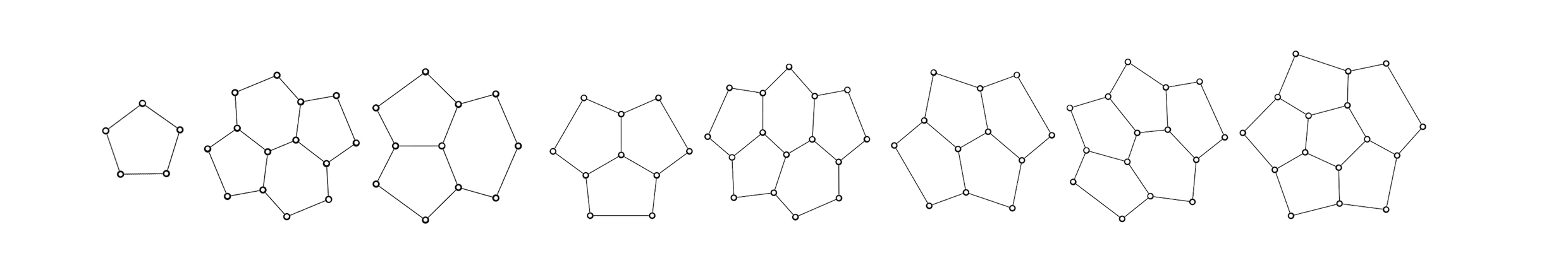
Nanocones are planar graphs with a majority of hexagonal faces, along with some non-hexagonal faces in core part. The non-hexagonal faces are typically pentagons, though they can also be triangles, squares, and other shapes. Different varieties of nanocones are produced based on the presence of different non-hexagonal faces in the core part of the nanocone structure. One of the major type is called as single \(k\)-gonal nanocone, whose structure is obtained by placing a cycle \(C_k\) with, \(k \geq 3\) vertices in the core and surrounding it with concentric layers of hexagons. Another type is obtained by differently positioning two or more pentagons in the core part and fencing it with concentric layers of hexagons. Nanocones with up to five pentagons in the core are defined and eight types of nanocone cores acknowledged in [5] are given in Figure 1.
In comparison to other carbon nanostructures, these one-dimensional carbon nanostructures have better porosity, outstanding conductivity, high yield, high chemical stability, high purity, low toxicities, and remarkable catalytic capabilities. These remarkable qualities make nanocones a viable substitute for carbon nanostructures. Thus, in a variety of applications, they offer a practical and beneficial substitute for carbon nanotubes and potentially graphene. Because of all these characteristics, it broadened its applicability to a number of domains, including biofuel cells, supercapacitors, gas storage devices, biochemical sensing, and electrochemical sensing [6-9]. A distinct collection of structural, mechanical, chemical, and electrical properties are defined by the nanocone’s geometry. Determining these qualities requires a substantial amount of work. This work, which models a compound’s structure as a chemical graph and then conducts quantitative analysis using molecular descriptors, has become quite efficient with the advent of chemical graph theory. With the aid of their corresponding molecular graph, this establishes a relationship between the physicochemical qualities and the structure of the chemical substances through some helpful graph invariants.
The idea of topological descriptors was first introduced by Wiener in 1947 [10]. Eventually many other topological descriptors were introduced following the pioneering works of Wiener [10] and Randić [11]. These include distance based descriptors, degree based descriptors, connectivity based descriptors, etc. Also the degree and distance was combined by Schultz [12] and Gutman [13] and they came up with degree-distance based descriptors. Each descriptor is related with distinct properties of a chemical structure and hence, these descriptors can be used to investigate the relationships between structure, properties and activity of chemical compounds. Pharmaceutical and chemical techniques are rapidly developing in the current technological development era, resulting in the rapid emergence of new medicines, nanomaterials, crystalline compounds, and so on. To investigate and analyse the physical, chemical or biological properties of these arising structures requires different chemical experiments and huge effort. Pharmaceutical and chemical researchers need to put in a great effort inorder to cover these vast area of research. The chemical structure’s molecular descriptor is a non-empirical numerical quantity that quantifies the structure and its diverging arrangement and these indices can be considered as a total function which draws the molecular structure to an actual number. The applications of certain distance based molecular descriptors are given in [10, 11, 14,17]. It has found its application in quantitative structure-property relationships and quantitative structure-activity relationships. An important application of QSPR/QSAR models is that the properties, activities, behavior, etc. of a newly developed or untested chemical compound can be inferred from the molecular structure of similar compounds whose properties, activities, characteristics, etc have already been evaluated.
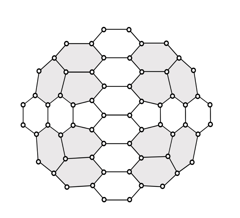
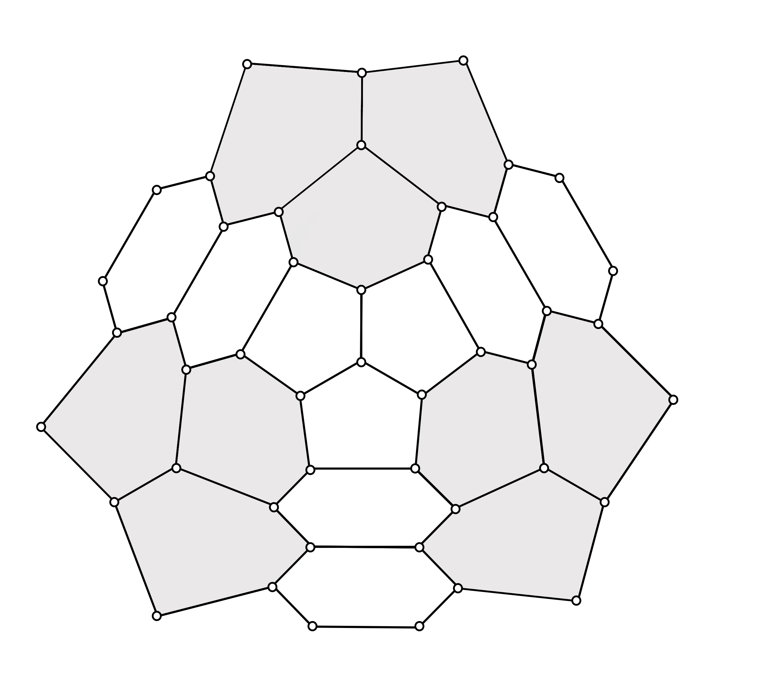
This paper considers carbon nanocones with two and three pentagons in their core. The pentagons are positioned in such a way that, the nanocone has symmetric configuration. Hence the nanocones are represented as \(CN_x^s(n): x \in \{2,3\}\) and \(n \geq 1\), where \('s'\) represents the symmetric configuration of the structure [18]. The nanocone with two pentagonal core fenced with two layers of hexagons, which is represented as \(CN_2^s(2)\) is presented in Figure 2 and the nanocone with three pentagonal core fenced with two layers of hexagons, which is denoted as \(CN_3^s(2)\) is given in Figure 3. The shaded portions in the figures (Figure 2 and Figure 3) evidently describes the symmetric configuration of the nanocone structures. The distance based descriptors for these symmetrically configured nanocone structures are determined in this study applying the technique of quotient graph approach. The quotient graph approach is initiated since regular cut method is not applicable as the molecular graph of the nanocone structures are not partial cubes. Various topological descriptors for single \(k\)-gonal nanocone were previously studied by researchers [19-22]. The saturation number of few nanocones were studied recently [18]. Also eccentricity based topological descriptors of carbon nanocones with two pentagons and three pentagons in the core of the nanocone were studied [23].
Consider a simple, finite, connected graph \(\zeta\) with vertex set, \(\mathbb{V}(\zeta)\) and edge set, \(\mathbb{E}(\zeta)\). The number of edges incident to a vertex \(\mu\) is the degree of that vertex and is denoted as \(d_{\mu}\). The shortest distance between any two vertices \(\mu, \nu \in \mathbb{V}(\zeta)\) is denoted as \(d_{\zeta} (\mu,\nu)\). The concepts of isometric subgraph, partial cubes, convex subgraph and Djoković-Winkler\((\Theta)\) relation are to be recollected while working on topological indices [24]. The Djoković-Winkler relation is a major concept applied in computing topological indices. For two edges \(\varepsilon=\mu \eta\) and \(\varrho=\kappa \nu\) of \(\zeta\), if \(d_{\zeta} (\eta,\nu)+d_{\zeta} (\mu,\kappa)\neq d_{\zeta} (\mu,\nu)+d_{\zeta} (\eta,\kappa)\), then we say \(\varepsilon\) is related to \(\varrho\). The relation \(\Theta\) is reflexive, symmetric and transitive in case of partial cubes. Its transitive closure \(\Theta^*\) forms an equivalence relation in general and partitions the edge set into convex components. Let \(\mathcal{F}=\{\mathcal{F}_1, \mathcal{F}_2,…\mathcal{F}_x\}\) be the \(\Theta^*\) equivalence class. A partition \(\mathfrak{E}=\{\xi_1, \xi_2, …, \xi_y\}\) of \(\mathbb{E}(G)\) is said to be coarser than partition \(\mathcal{F}\) if each set \(\xi_i\) is the union of one or more \(\Theta^*\)-classes of \(G\).
The concept of strength weighted graph is presented in [24]. A strength weighted graph is denoted as \(\zeta_{sw}=(\zeta,[w_v,s_v ],s_e)\), whose vertex weight, vertex strength and edge strength are denoted as \(w_v\), \(s_v\) and \(s_e\) respectively. For convenience, let us consider strength-weighted graph \(\zeta_{sw}\) as \(\zeta\). For an edge \(\varepsilon=\mu \eta\), the sets \(N_{\mu}(\varepsilon|\zeta)=\{\lambda \in \mathbb{V}(\zeta):d_{\zeta} (\mu,\lambda)<d_{\zeta} (\eta,\lambda)\}\) and \(M_{\mu}(\varepsilon|\zeta)=\{\chi \in \mathbb{E}(\zeta):d_{\zeta} (\mu,\chi)<d_{\zeta} (\eta,\chi)\}\). The cardinality of sets \(N_{\mu}(\varepsilon|\zeta)\) and \(M_{\mu}(\varepsilon|\zeta)\) are described as follows: \[n_{\mu}(\varepsilon|\zeta)=\displaystyle \sum_{\lambda \in N_{\mu}(\varepsilon|\zeta)}w_v (\lambda)\] and \[m_{\mu}(\varepsilon|\zeta)= \displaystyle \sum_{\lambda \in N_{\mu}(\varepsilon|\zeta)}s_v (\lambda)+\displaystyle \sum_{\chi \in M_{\mu}(\varepsilon|\zeta)}s_e (\chi)\] respectively.
The values of \(n_{\eta}(\varepsilon|\zeta)\) and \(m_{\eta}(\varepsilon|\zeta)\) are analogous. For more basic terminologies and definitions refer to [24,25].
The distance based molecular descriptors and their corresponding mathematical expression for strength-weighted graph \(\zeta\) [24] are given in Table 1.
| Wiener | \(W(\zeta)=\displaystyle \sum_{\{\mu,\eta\}\subseteq \mathbb{V}(\zeta)}w_v (\mu) w_v (\eta) d_\zeta (\mu,\eta)\) |
|---|---|
| Szeged | \(Sz_v (\zeta)=\displaystyle \sum_{\varepsilon=\mu\eta \in \mathbb{E}(\zeta)}s_e (\varepsilon)n_{\mu} (\varepsilon|\zeta) n_{\eta} (\varepsilon|\zeta)\) |
| Edge-Szeged | \(Sz_e (\zeta)=\displaystyle\sum_{\varepsilon=\mu\eta \in \mathbb{E}(\zeta)}s_e (\varepsilon)m_{\mu} (\varepsilon|\zeta)m_{\eta} (\varepsilon|\zeta)\) |
| Mostar | \(Mo(G)=\displaystyle \sum_{\varepsilon=\mu\eta \in \mathbb{E}(\zeta)}s_e (\varepsilon)|n_{\mu}(\varepsilon|\zeta)-n_{\eta} (\varepsilon|\zeta)|\) |
| Edge-Mostar | \(Mo_e (G)=\displaystyle \sum_{\varepsilon=\mu\eta \in \mathbb{E}(\zeta)}s_e (\varepsilon)|m_{\mu} (\varepsilon|\zeta)-m_{\eta} (\varepsilon|\zeta)|\) |
| Padmakar-Ivan | \(PI(\zeta)=\displaystyle \sum_{\varepsilon=\mu\eta \in \mathbb{E}(\zeta)}s_e (\varepsilon)[m_{\mu} (\varepsilon|\zeta)+m_{\eta}\} (\varepsilon|\zeta)]\) |
This section comprises of theorems based on the distance based molecular descriptors of symmetrically configured two pentagonal nanocone, \(CN_2^s(n), n\geq 1\) and symmetrically configured three pentagonal nanocone, \(CN_3^s(n), n\geq 1\). For the computation, the quotient graph approach is used, since usual cut method is not applicable as the corresponding molecular graphs are not partial cubes. In this approach, the original graphs are converted into quotient graphs with the help of \(\Theta^*\)– classes. Further, the descriptors of each quotient graphs are determined and are added up correspondingly inorder to obtain the descriptors of original graph. This transformation shrinks the original graphs into smaller graphs, which makes the computation easier and faster.
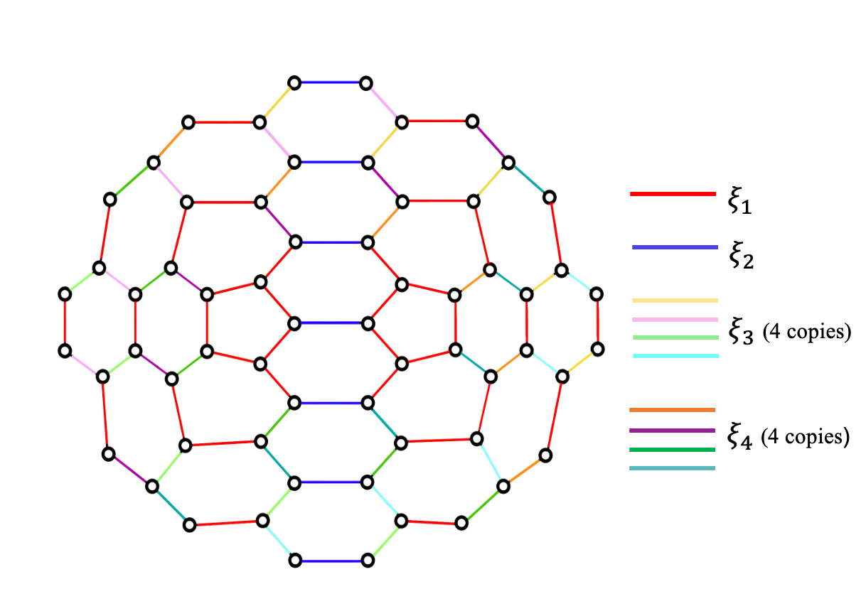
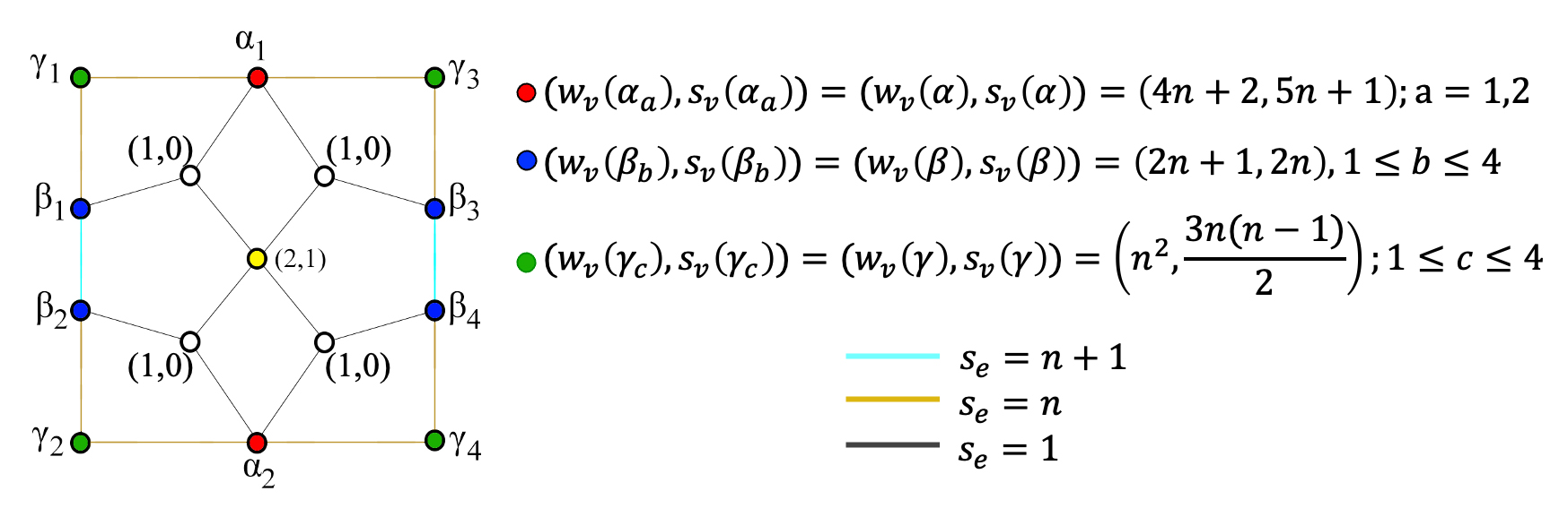
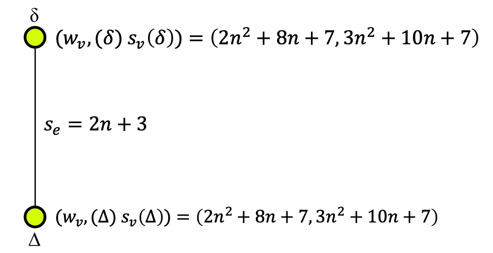
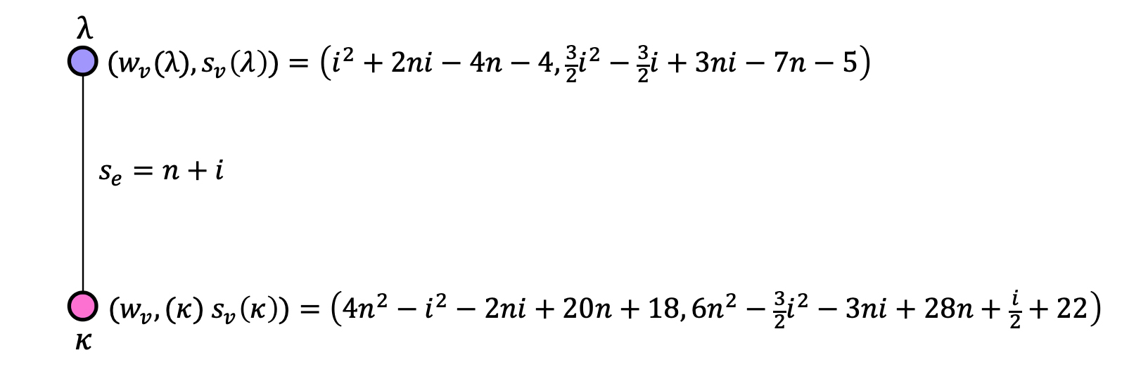
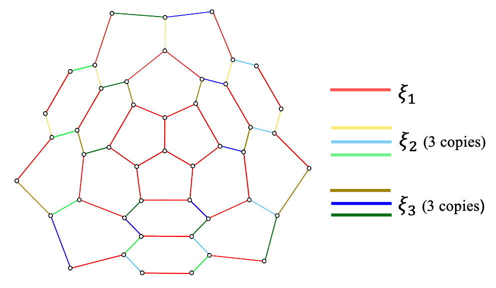
The symmetrically configured two pentagonal nanocone, \(CN_2^s(n), n \geq 1\)has \(4 n^2+16 n +14\) vertices and \(6n^2+22n +17\) edges. Applying the Djoković-Winkler relation, the \(\Theta^*\)– classes of \(CN_2^s(n)\) are determined and based on the same, \(CN_2^s(n)\) can have \(4n+2\) quotient graphs, namely \(CN_2^s/\xi_1\), \(CN_2^s/\xi_2\) and \(CN_2^s/\xi_i, 3\leq i \leq 4n+2\), where \(\xi_j, 1\leq j \leq 4n+2\) are the \(\Theta^*\)– classes. The \(\Theta^*\)– classes of \(CN_2^s(2)\) is presented in Figure 4. In general, there are three types of quotient graphs for \(CN_2^s\), \(CN_2^s/\xi_1\), \(CN_2^s/\xi_2\) and \(CN_2^s/\xi_i, 3\leq i \leq n+2\), which are illustrated in Figure 5, Figure 6 and Figure 7 respectively. Also there are four copies of the third type of quotient graph \(CN_2^s/\xi_i\).
Theorem 1. For \(n\geq1\), \[\begin{aligned} &W(CN_2^s(n))=\frac{56}{5} \hspace{0.05cm} n^5 + 118 \hspace{0.05cm} n^4 + 448 \hspace{0.05cm} n^3 + 820 \hspace{0.05cm} n^2 + \frac{3594}{5} \hspace{0.05cm} n + 243. \end{aligned}\]
Proof. The nanocone structure \(CN_2^s(n)\) has three types of quotient graphs \(CN_2^s/\xi_1\), \(CN_2^s/\xi_2\) and \(CN_2^s/\xi_i, 3\leq i \leq n+2\), as shown in Figure 5, Figure 6 and Figure 7 respectively.
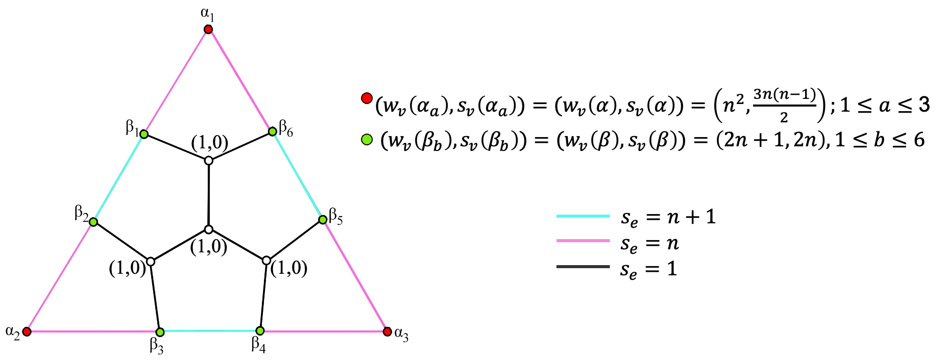
For the quotient graph \(CN_2^s/\xi_1\) (Figure 5), the transmission index method [26] can be applied to compute the wiener index. Therefore, \[\begin{aligned} W(CN_2^s/\xi_1) =& \frac{T(\mu)}{2}, \text{where } \mu \in \mathbb{V}(CN_2^s/\xi_1) \text{ and } T(\mu) \text{ is the transmission index of $\mu$.}\\ =&4 (w_v(\alpha))^2+18 (w_v(\beta))^2+20 (w_v(\gamma))^2+24w_v(\alpha)+52w_v(\beta)\\&+68w_v(\gamma)+20w_v(\alpha)w_v(\beta)+40w_v(\beta) w_v(\gamma)+20w_v(\alpha) w_v(\gamma)+20, \end{aligned}\] where \(w_v(\alpha)=4n+2, w_v(\beta)= 2n+1, w_v(\gamma)=n^2.\) Hence, \(W(CN_2^s/\xi_1)=20 n^4 + 160 n^3 + 444 n^2 + 496 n + 194\).
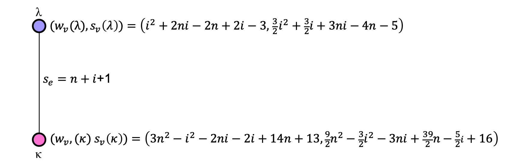
Considering the second type of quotient graph \(CN_2^s/\xi_2\) (Figure 6), the wiener index can be computed as follows: \[\begin{aligned} W(CN_2^s/\xi_2)&=w_v(\delta) \times w_v(\Delta), \text{where, } w_v(\delta)=w_v(\Delta)=2n^2+8n+7\\ &=(2n^2+8n+7)^2. \end{aligned}\] For the quotient graph \(CN_2^s/\xi_i, 3\leq i \leq n+2\) (Figure 7), considering the four copies of the quotient graph, the wiener index can be computed as follows. \[\begin{aligned} W(CN_2^s/\xi_i)&=4\times w_v(\lambda) \times w_v(\kappa), \\ &=4(i^2+2ni-4n-4)(4n^2-i^2-2ni+20n+18), \end{aligned}\] where, \(w_v(\lambda)=i^2+2ni-4n-4,\) \(w_v(\kappa)=4n^2-i^2-2ni+20n+18.\) Hence, \(\displaystyle \sum_{i=3}^{n+2} W(CN_2^s/\xi_i)=\frac{2n}{5}\hspace{0.05cm} (28 n^4 + 235 n^3 + 640 n^2 + 710 n + 277)\).
By using ([24]-Theorem 1), the wiener index of \(CN_2^s(n)\) can be determined as follows: \[\begin{aligned} W(CN_2^s(n))&= W(CN_2^s/\xi_1)+W(CN_2^s/\xi_2)+\sum_{i=3}^{n+2} W(CN_2^s/\xi_i)\\ &= \frac{56}{5} \hspace{0.05cm} n^5 + 118 \hspace{0.05cm} n^4 + 448 \hspace{0.05cm} n^3 + 820 \hspace{0.05cm} n^2 + \frac{3594}{5} \hspace{0.05cm} n + 243. \end{aligned}\] ◻
Theorem 2. For \(n\geq1\), \[\begin{aligned} &Sz_v(CN_2^s(n))=18 \hspace{0.05cm} n^6 + 220 \hspace{0.05cm} n^5 + 983 \hspace{0.05cm} n^4 + 2256 \hspace{0.05cm} n^3 + 2871 \hspace{0.05cm} n^2 + 1934 \hspace{0.05cm} n + 539.\\ &Sz_e(CN_2^s(n))=\frac{81}{2} \hspace{0.05cm} n^6 + \frac{4349}{10} \hspace{0.05cm} n^5 + \frac{5050}{3} \hspace{0.05cm} n^4 + \frac{20623}{6} \hspace{0.05cm} n^3 + \frac{23899}{6} \hspace{0.05cm} n^2 + \frac{37199}{15} \hspace{0.05cm} n + 645. \end{aligned}\]
Proof. As mentioned, \(CN_2^s(n)\) has three types of quotient graphs \(CN_2^s\), \(CN_2^s/\xi_1\), \(CN_2^s/\xi_2\) and \(CN_2^s/\xi_i, 3\leq i \leq n+2\), as given in Figure 5, Figure 6 and Figure 7 respectively. From Table 1, \[\begin{aligned} Sz_v (\zeta)=\sum_{\varepsilon=\mu\eta \in \mathbb{E}(\zeta)}s_e (\varepsilon)n_{\mu} (\varepsilon|\zeta) n_{\eta} (\varepsilon|\zeta). \end{aligned}\]
For quotient graph \(CN_2^s/\xi_1\) (Figure 5), \[\begin{aligned} Sz_v(CN_2^s/\xi_1)&=\sum_{\varepsilon=\mu\eta \in \mathbb{E}(CN_2^s/\xi_1)}s_e (\varepsilon)n_{\mu} (\varepsilon|(CN_2^s/\xi_1)) n_{\eta} (\varepsilon|(CN_2^s/\xi_1))\\ & = 32 n^5 + 264 n^4 + 904 n^3 + 1520 n^2 + 1240 n + 392. \end{aligned}\]
For quotient graph \(CN_2^s/\xi_2\) (Figure 6), \[\begin{aligned} Sz_v(CN_2^s/\xi_2)&=\sum_{\varepsilon=\mu\eta \in \mathbb{E}(CN_2^s/\xi_2)}s_e (\varepsilon)n_{\mu} (\varepsilon|(CN_2^s/\xi_2)) n_{\eta} (\varepsilon|(CN_2^s/\xi_2))\\ & = (2n+3) \{ w_v(\delta) \times w_v(\Delta)\}, \text{where, } w_v(\delta)=w_v(\Delta)=2n^2+8n+7\\ &=(2n+3)\{(2n^2+8n+7)^2\}. \end{aligned}\]
For quotient graph \(CN_2^s/\xi_i, 3\leq i \leq n+2\) (Figure 7), considering four copies of the quotient graph, \[\begin{aligned} Sz_v(CN_2^s/\xi_i)&=\sum_{\varepsilon=\mu\eta \in \mathbb{E}(CN_2^s/\xi_i)}s_e (\varepsilon)n_{\mu} (\varepsilon|(CN_2^s/\xi_i)) n_{\eta} (\varepsilon|(CN_2^s/\xi_i))\\ & = 4 (n+i) \{ w_v(\lambda) \times w_v(\kappa)\}, \\ &=4(n+i)\{(i^2+2ni-4n-4)(4n^2-i^2-2ni+20n+18)\}. \end{aligned}\] where, \(w_v(\lambda)=i^2+2ni-4n-4, w_v(\kappa)=4n^2-i^2-2ni+20n+18.\) Hence, \(\displaystyle \sum_{i=3}^{n+2} Sz_v(CN_2^s/\xi_i)=n (18 n^5 + 180 n^4 + 643 n^3 + 1072 n^2 + 851 n + 260)\)
By using ([24]-Theorem 1), the szeged index of \(CN_2^s(n)\) is, \[\begin{aligned} SZ_v(CN_2^s(n))&= Sz_v(CN_2^s/\xi_1)+Sz_v(CN_2^s/\xi_2)+\sum_{i=3}^{n+2} Sz_v(CN_2^s/\xi_i)\\ &=18 \hspace{0.05cm} n^6 + 220 \hspace{0.05cm} n^5 + 983 \hspace{0.05cm} n^4 + 2256 \hspace{0.05cm} n^3 + 2871 \hspace{0.05cm} n^2 + 1934 \hspace{0.05cm} n + 539. \end{aligned}\]
Similarly using the expression for computing the edge-szeged index from Table 1, the following can be determined: \[\begin{aligned} Sz_e(CN_2^s/\xi_1)&=\sum_{\varepsilon=\mu\eta \in \mathbb{E}(CN_2^s/\xi_1)}s_e (\varepsilon)m_{\mu} (\varepsilon|(CN_2^s/\xi_1)) m_{\eta} (\varepsilon|(CN_2^s/\xi_1))\\ & = 72 \hspace{0.05cm} n^5 + 534 \hspace{0.05cm} n^4 + 1716 \hspace{0.05cm} n^3 + 2638 \hspace{0.05cm} n^2 + 1886 \hspace{0.05cm} n + 498. \end{aligned}\] \[\begin{aligned} Sz_e(CN_2^s/\xi_2)&=\sum_{\varepsilon=\mu\eta \in \mathbb{E}(CN_2^s/\xi_2)}s_e (\varepsilon)m_{\mu} (\varepsilon|(CN_2^s/\xi_2)) m_{\eta} (\varepsilon|(CN_2^s/\xi_2))\\ & = (2n+3)\{ s_v(\delta) \times s_v(\Delta)\}, \\ &=(2n + 3) \{(3 n^2 + 10 n + 7)^2\}, \end{aligned}\] where, \(s_v(\delta)=s_v(\Delta)=3 n^2 + 10 n + 7.\) \[\begin{aligned} Sz_e(CN_2^s/\xi_i)&=\sum_{\varepsilon=\mu\eta \in \mathbb{E}(CN_2^s/\xi_i)}s_e (\varepsilon)m_{\mu} (\varepsilon|(CN_2^s/\xi_i)) m_{\eta} (\varepsilon|(CN_2^s/\xi_i))\\ & = 4 (n+i) \{ s_v(\lambda) \times s_v(\kappa)\}, \\ &= 4(n+i)\bigg\{\bigg(\frac{3 i^2}{2}-\frac{3 i}{2}+3ni-7n-5\bigg) \bigg(6 n^2-\frac{3 i^2}{2} -3ni+28n+\frac{i}{2}+22\bigg)\bigg\},\\ \sum_{i=3}^{n+2}(Sz_e(CN_2^s/\xi_i))&= \frac{n}{30}(1215 n^5 + 10347 n^4 + 30070 n^3 + 37715 n^2 + 19175 n + 2278), \end{aligned}\] where, \(s_v(\lambda)=\frac{3 i^2}{2}-\frac{3 i}{2}+3ni-7n-5, s_v(\kappa)=6 n^2-\frac{3 i^2}{2} -3ni+28n+\frac{i}{2}+22.\) By using ([24]-Theorem 1), \[\begin{aligned} Sz_e(CN_2^s(n))&= Sz_e(CN_2^s/\xi_1)+Sz_e(CN_2^s/\xi_2)+\sum_{i=3}^{n+2} Sz_e(CN_2^s/\xi_i)\\ &=\frac{81}{2} \hspace{0.05cm} n^6 + \frac{4349}{10} \hspace{0.05cm} n^5 + \frac{5050}{3} \hspace{0.05cm} n^4 + \frac{20623}{6} \hspace{0.05cm} n^3 + \frac{23899}{6} \hspace{0.05cm} n^2 + \frac{37199}{15} \hspace{0.05cm} n + 645. \end{aligned}\] ◻
Theorem 3. For \(n\geq1\), \[\begin{aligned} Mo(CN_2^s(n))=&4 | 7+4n-n^2| + (4 n+8) | 5+2n-n^2| +16 n^2+28 n\\&+\sum_{i=3}^{n+2}\bigg(4(n+i)|4 n^2 – 2 i^2 – 4ni + 24n + 22|\bigg).\\ Mo_e(CN_2^s(n))=&(4n+8)|2n – \frac{3}{2} n(n – 1) + 7| + 4|5n – \frac{3}{2} n(n – 1) + 10| + 20 n^2 + 40 n\\&+\sum_{i=3}^{n+2}\bigg(4(n+i)| 6 n^2- 3 i^2 – 6 n i + 2 i + 35 n + 27|\bigg).\\ PI(CN_2^s(n))=&36 \hspace{0.05cm} n^4 + \frac{746}{3} \hspace{0.05cm} n^3 + 586 \hspace{0.05cm} n^2 + \frac{1870}{3} \hspace{0.05cm} n + 238. \end{aligned}\]
Proof. \(CN_2^s(n)\) has three types of quotient graphs \(CN_2^s\), \(CN_2^s/\xi_1\), \(CN_2^s/\xi_2\) and \(CN_2^s/\xi_i, 3\leq i \leq n+2\), as given in Figure 5, Figure 6 and Figure 7 respectively. From Table 1, \[\begin{aligned} Mo(\zeta)=\sum_{\varepsilon=\mu\eta \in \mathbb{E}(\zeta)}s_e (\varepsilon)|n_{\mu} (\varepsilon|\zeta) – n_{\eta} (\varepsilon|\zeta)|. \end{aligned}\]
For quotient graph \(CN_2^s/\xi_1\) (Figure 5), \[\begin{aligned} Mo(CN_2^s/\xi_1)&=\sum_{\varepsilon=\mu\eta \in \mathbb{E}(CN_2^s/\xi_1)}s_e (\varepsilon)\big|n_{\mu} (\varepsilon|(CN_2^s/\xi_1)) – n_{\eta} (\varepsilon|(CN_2^s/\xi_1))\big|\\ & = 4 \hspace{0.05cm} | 7+4n-n^2| + (4 n+8) \hspace{0.05cm} | 5+2n-n^2| +16 n^2+28 n. \end{aligned}\]
For quotient graph \(CN_2^s/\xi_2\) (Figure 6), \[\begin{aligned} Mo(CN_2^s/\xi_2)&=\sum_{\varepsilon=\mu\eta \in \mathbb{E}(CN_2^s/\xi_2)}s_e (\varepsilon) \big|n_{\mu} (\varepsilon|(CN_2^s/\xi_2))- n_{\eta} (\varepsilon|(CN_2^s/\xi_2))\big|\\ & = (2n+3)\times |w_v(\delta) – w_v(\Delta)| \\ &=(2n+3)(0)=0, \end{aligned}\] where, \(w_v(\delta)=w_v(\Delta)=2n^2+8n+7.\)
For quotient graph \(CN_2^s/\xi_i, 3\leq i \leq n+2\) (Figure 7), considering four copies of the quotient graph, \[\begin{aligned} Mo(CN_2^s/\xi_i)&=\sum_{\varepsilon=\mu\eta \in \mathbb{E}(CN_2^s/\xi_i)}s_e (\varepsilon)\big|n_{\mu} (\varepsilon|(CN_2^s/\xi_i)) – n_{\eta} (\varepsilon|(CN_2^s/\xi_i))\big|\\ & = 4 (n+i) \times |w_v(\lambda) – w_v(\kappa)|, \\ &=4(n+i) \hspace{0.05cm} \big|4 n^2 – 2 i^2 – 4ni + 24n + 22\big|, \end{aligned}\] where, \(w_v(\lambda)=i^2+2ni-4n-4, w_v(\kappa)=4n^2-i^2-2ni+20n+18.\) Hence, \(\displaystyle \sum_{i=3}^{n+2} Mo(CN_2^s/\xi_i)=\displaystyle \sum_{i=3}^{n+2}\bigg(4(n+i) \hspace{0.05cm} \big|4 n^2 – 2 i^2 – 4ni + 24n + 22\big|\bigg)\).
By using ([24]-Theorem 1), the mostar index of \(CN_2^s(n)\) is, \[\begin{aligned} Mo(CN_2^s(n))=& Mo(CN_2^s/\xi_1)+Mo(CN_2^s/\xi_2)+\sum_{i=3}^{n+2} Mo(CN_2^s/\xi_i)\\ =&4 \hspace{0.05cm} \big| 7+4n-n^2\big| + (4 n+8)\hspace{0.05cm} \big| 5+2n-n^2\big| +16 n^2+28 n\\&+\sum_{i=3}^{n+2}\bigg(4(n+i) \hspace{0.05cm} \big|4 n^2 – 2 i^2 – 4ni + 24n + 22\big|\bigg). \end{aligned}\] Similarly using the expression for computing the edge-mostar index from Table 1, the following can be determined. \[\begin{aligned} Mo_e(CN_2^s/\xi_1)&=\sum_{\varepsilon=\mu\eta \in \mathbb{E}(CN_2^s/\xi_1)}s_e (\varepsilon)\big|m_{\mu} (\varepsilon|(CN_2^s/\xi_1)) – m_{\eta} (\varepsilon|(CN_2^s/\xi_1))\big|\\ & = (4n+8) \hspace{0.05cm} \big|2n – \frac{3}{2} n(n – 1) + 7\big| + 4 \hspace{0.05cm} \big|5n – \frac{3}{2} n(n – 1) + 10\big| + 20 n^2 + 40 n.\\ Mo_e(CN_2^s/\xi_2)&=\sum_{\varepsilon=\mu\eta \in \mathbb{E}(CN_2^s/\xi_2)}s_e (\varepsilon)\big|m_{\mu} (\varepsilon|(CN_2^s/\xi_2)) – m_{\eta} (\varepsilon|(CN_2^s/\xi_2))\big|\\ & = (2n+3)\times \big|s_v(\delta) – s_v(\Delta)\big|, \\ &=(2n + 3) (0)=0. \end{aligned}\] where, \(s_v(\delta)=s_v(\Delta)=3 n^2 + 10 n + 7.\) \[\begin{aligned} Mo_e(CN_2^s/\xi_i)&=\sum_{\varepsilon=\mu\eta \in \mathbb{E}(CN_2^s/\xi_i)}s_e (\varepsilon)\big|m_{\mu} (\varepsilon|(CN_2^s/\xi_i)) – m_{\eta} (\varepsilon|(CN_2^s/\xi_i))\big|\\ & = 4 (n+i) \times \big|s_v(\lambda) – s_v(\kappa)\big|, \\ &= 4(n+i) \hspace{0.05cm} \big| 6 n^2- 3 i^2 – 6 n i + 2 i + 35 n + 27\big|\\ \sum_{i=3}^{n+2}(Mo_e&(CN_2^s/\xi_i))= \sum_{i=3}^{n+2}\bigg(4(n+i) \hspace{0.05cm} \big| 6 n^2- 3 i^2 – 6 n i + 2 i + 35 n + 27\big|\bigg). \end{aligned}\] where, \(s_v(\lambda)=\frac{3 i^2}{2}-\frac{3 i}{2}+3ni-7n-5, s_v(\kappa)=6 n^2-\frac{3 i^2}{2} -3ni+28n+\frac{i}{2}+22.\) Hence by using ([24]-Theorem 1), \[\begin{aligned} Mo_e(CN_2^s(n))=& Mo_e(CN_2^s/\xi_1)+Mo_e(CN_2^s/\xi_2)+\sum_{i=3}^{n+2} Mo_e(CN_2^s/\xi_i)\\ =&(4n+8) \hspace{0.05cm} \big|2n – \frac{3}{2} n(n – 1) + 7 \big| + 4 \hspace{0.05cm} \big|5n – \frac{3}{2} n(n – 1) + 10\big| + 20 n^2 + 40 n\\&+\sum_{i=3}^{n+2}\bigg(4(n+i) \hspace{0.05cm} \big| 6 n^2- 3 i^2 – 6 n i + 2 i + 35 n + 27\big|\bigg). \end{aligned}\] In the similar pattern, using the expression \(PI(\zeta)=\displaystyle \sum_{\varepsilon=\mu\eta \in \mathbb{E}(\zeta)}s_e (\varepsilon)[m_{\mu} (\varepsilon|\zeta)+m_{\eta} (\varepsilon|\zeta)]\), \[\begin{aligned} PI(CN_2^s/\xi_1) &= 54 n^3 + 236 n^2 + 390 n + 196,\\ PI(CN_2^s/\xi_2)&=(2 n + 3) (6 n^2 + 20 n + 14),\\ PI(CN_2^s/\xi_i)&=4 (n+ i) (6 n^2 + 21 n – i + 17),\\ \sum_{i=3}^{n+2}(PI(CN_2^s/\xi_i))&=\frac{4 n}{3} (27 n^3 + 137 n^2 + 219 n + 109). \end{aligned}\] Hence, \[\begin{aligned} PI(CN_2^s(n))&= PI(CN_2^s/\xi_1)+PI(CN_2^s/\xi_2)+\sum_{i=3}^{n+2} PI(CN_2^s/\xi_i)\\ &=36 \hspace{0.05cm} n^4 + \frac{746}{3} \hspace{0.05cm} n^3 + 586 \hspace{0.05cm} n^2 + \frac{1870}{3} \hspace{0.05cm} n + 238 . \end{aligned}\] ◻
The symmetrically configured three pentagonal nanocone, \(CN_3^s(n), n\geq 1\) has \(3 n^2+12 n +10\) vertices and \(\displaystyle \frac{9}{2} n^2+\frac{33}{2} n +12\) edges. Based on the \(\Theta^*\)– classes of \(CN_3^s(n)\), the original graph can have \(3n+1\) quotient graphs, namely \(CN_3^s/\xi_1\) and \(CN_3^s/\xi_i, 2\leq i \leq 3n+1\), where \(\xi_j, 1\leq j \leq 3n+1\) are the \(\Theta^*\)– classes of the original graph. The \(\Theta^*\)– classes of \(CN_3^s(2)\) is presented in Figure 8. For each \(i\), there are three copies of the quotient graph \(CN_3^s/\xi_i\). Therefore, in general, \(CN_3^s(n)\) have two types of quotient graphs, \(CN_3^s/\xi_1\), \(CN_3^s/\xi_i, 2\leq i \leq n+1\), which are illustrated in Figure 9 and Figure 10 respectively.
Theorem 4. For \(n\geq1\), \[\begin{aligned} &W(CN_3^s(n))= \frac{22}{5} \hspace{0.05cm} n^5 + 53 \hspace{0.05cm} n^4 + \frac{423}{2} \hspace{0.05cm} n^3 + 376 \hspace{0.05cm} n^2 + \frac{3091}{10} \hspace{0.05cm} n + 96 \end{aligned}\]
Proof. The proof follows the similar pattern as in Theorem 1. ◻
Theorem 5. For \(n\geq1\), \[\begin{aligned} & Sz_v(CN_3^s(n))= \frac{27}{4} \hspace{0.05cm} n^6 + 96 \hspace{0.05cm} n^5 + 459 \hspace{0.05cm} n^4 + 1044 \hspace{0.05cm} n^3 + \frac{4881}{4} \hspace{0.05cm} n^2 + 711 \hspace{0.05cm} n + 165. \\& Sz_e(CN_3^s(n))=\frac{243}{16} \hspace{0.05cm} n^6 + \frac{15069}{80} \hspace{0.05cm} n^5 + \frac{12655}{16} \hspace{0.05cm} n^4 + \frac{25367}{16} n^3 + \frac{13327}{8}\hspace{0.05cm} n^2 + \frac{4571}{5} \hspace{0.05cm} n + 216. \end{aligned}\]
Proof. The nanocone \(CN_3^s(n)\) have two types of quotient graphs, \(CN_3^s/\xi_1\), \(CN_3^s/\xi_i, 2\leq i \leq n+1\) (Figure 9 and Figure 10 respectively) and there are three copies of the later type. The remaining proof is as in Theorem 2. ◻
Theorem 6. For \(n\geq1\), \[\begin{aligned} Mo(CN_3^s(n))= &(6n+6) \hspace{0.05cm} \big| 4+2n – n^2\big| + 3 \hspace{0.05cm} \big|n^2 – 2\big| \\&+\sum_{i=2}^{n+1} \bigg(3(n+i+1) \hspace{0.05cm} \big|2 i^2 + 4 n i + 4 i – 3 n^2 – 16 n – 16\big| \bigg). \\ Mo_e(CN_3^s(n))=&3 \hspace{0.05cm} \big| n + \frac{3}{2} n (n – 1) – 3\big| + 6 \hspace{0.05cm} \big| n – \frac{3}{2} n (n – 1) + 5 \big| + 6 n \hspace{0.05cm} \big|2 n – \frac{3}{2} n (n – 1) + 6\big| \\&+ \sum_{i=2}^{n+1} \bigg(3(n+i+1) \hspace{0.05cm} \big|4 i – \frac{47 n}{2} + 6 n i + 3 i^2 – \frac{9 n^2}{2} – 21\big| \bigg). \\PI(CN_3^s(n))=&\frac{81}{4} \hspace{0.05cm} n^4 + 137 \hspace{0.05cm} n^3 + \frac{1311}{4} \hspace{0.05cm} n^2 + 322 \hspace{0.05cm} n + 111. \end{aligned}\]
Proof. The quotient graphs of \(CN_3^s(n)\) are \(CN_3^s/\xi_1\) (Figure 9) and \(CN_3^s/\xi_i, 2\leq i \leq n+1\) (Figure 10) and there are three copies of the later type. The remaining proof is similar to proof of Theorem 3. ◻
Investigation a chemical structure experimentally is time consuming as well as cost consuming. Determining molecular descriptors of the chemical structure eases the procedure and is found to be an effective way to analyse the structure. In this work, the distance based molecular descriptors for symmetrically configured two pentagonal nanocone, \(CN_2^s(n), n\geq 1\) and symmetrically configured three pentagonal nanocone, \(CN_3^s(n), n\geq 1\) are determined using a convincing technique, known as the quotient graph approach. When compared to other nanoparticles like nanotubes, graphene, etc., nanocones have unique features that make them a viable substitute for those nanostructures. This research contributes to the understanding of several nanocone structural features that are useful in a variety of industries. Additionally, the graphical depiction could support a comparison analysis of the structure’s different attributes.
The authors did not receive support from any organization for the submitted work.
Authors declare no conflict of interest.