
With the rapid advancements in remote sensing technology and satellite equip-ment performance, satellite imagery has gained significant importance in various ap-plications[1,2]. These applications include Earth observation, climate change analysis, and environmental monitoring[3,4]. Clouds can often contaminate optical re-mote-sensing images. Extensive data from the International Satellite Cloud Climatology Project (ISCCP) reveals that clouds typically cover nearly two-thirds of the Earth’s sur-face [5]. Cloud occlusion poses a substantial challenge in optical imagery, as both clouds and their shadows obstruct ground information and degrade the quality of the images[6]. Consequently, this hampers the utilization and quality of the image data, thus lim-iting their applicability in further research and applications [7,8]. Therefore, removing clouds to enhance the utilization of optical remote-sensing images becomes necessary.
In recent years, cloud removal research has gained considerable attention, devel-oping numerous methods and algorithms. There are two main categories of approaches: traditional and deep learning-based [9,10]. Traditional methods include Dark Channel Prior (DCP)[11], homomorphic filters [12], and wavelet transforms [13]. These highly interpretable techniques are easy to implement, leading to widespread adoption. However, traditional approaches need help generalizing processing methods for thin and thick clouds, relying on prior knowledge and manually extracting feature infor-mation, thereby limiting their applicability in certain regions [14].
Deep learning techniques have significantly progressed in detecting and removing clouds [15,16]. For instance, Convolutional Neural Networks (CNNs) have been exten-sively employed to address the cloud removal problem, offering distinct advantages in automatically extracting feature information [17]. Chen et al. [18] proposed end-to-end CNN architectures that effectively remove both thick clouds and cloud shadows sim-ultaneously. This approach demonstrates the power of CNNs in tackling complex cloud patterns. In addition to CNNs, generative adversarial networks (GANs) have gained prominence in deep learning research. Enomoto et al. [19] employed multispectral con-ditional GANs (McGANs) to recover cloud-contaminated regions by synthesizing sim-ulated clouds on cloudless ground truth images as input data. However, the study re-vealed that the simulated clouds differ somewhat from real clouds, highlighting the challenges in accurately modeling cloud behavior. Another study by Darbaghshahi et al. [5] utilized two GAN architectures to identify and eliminate clouds in satellite im-agery. They utilized the Super-Resolution Generative Adversarial Network (SRGAN), initially designed for image super-resolution, to eliminate clouds from optical remote sensing images. Additionally, the Pixel to Pixel (pix2pix) Conditional GAN (cGAN) approach was applied to restore cloud-free optical images in a cropland time series [20]. It is important to note that these deep learning-based methods heavily rely on the quality of the input data, and the success of deep learning techniques in cloud detection and removal underscores the significance of reliable and diverse cloud datasets. A well-curated dataset plays a pivotal role in enabling models to learn robust representa-tions of clouds and their variations, thus leading to improved accuracy in cloud removal tasks [21].
Constructing a comprehensive cloud dataset that encompasses both authentic cloud instances and their cloud-free counterparts is a daunting and intricate endeavor [22]. However, the existing body of literature offers a range of published manually la-beled cloud datasets that can be effectively employed. One prominent example is the SEN1-2 dataset, introduced by Schmitt et al. [23]. These patch-pairs were acquired using the Sentinel-1 Synthetic Aperture Radar (SAR) and Sentinel-2 optical sensors, thereby capturing diverse optical images in cloudless and cloudy conditions [24]. These patches were meticulously gathered from the Google Earth Engine platform, encompassing various land masses across the globe and representing all four seasons. SEN12MS-CR [25] dataset and SEN12MS-CR-TS [26] dataset was proposed in 2021 and 2022, respec-tively. SEN12MS-CR-TS dataset comprises cloud-free and cloudy Sentinel-2 multitem-poral images and incorporates a comprehensive one-year-long time series of Sentinel-1 satellite observations. Including multitemporal data in this dataset offers a unique op-portunity to investigate and analyze temporal changes and variations in cloud cover over extended periods. Furthermore, Li et al. [27] have released the WHUS2-CR dataset, which features paired images exhibiting minimal temporal gaps between cloud-free and cloudy Sentinel-2A images. This dataset serves as a valuable resource for studying the immediate effects of cloud cover on observed imagery, enabling researchers to delve into the intricacies of cloud-induced image alterations.
It is worth noting that manually labeled cloud datasets are the gold standard for evaluating the performance of diverse algorithms in satellite image analysis [28,29]. These datasets serve as a fundamental reference point, allowing researchers to rigor-ously assess the accuracy and effectiveness of their algorithms in tasks such as cloud detection and removal. By utilizing these datasets, researchers can establish a bench-mark for comparison, facilitating the development of robust cloud removal techniques that can substantially enhance the quality and reliability of satellite imagery analysis. However, the availability of publicly accessible manually labeled datasets for cloud removal is limited, primarily due to the time-consuming nature of this task.
To address these challenges and limitations of previous studies, this paper intro-duces several contributions aimed at advancing the progress of deep learning tech-niques in cloud removal from remote sensing images.
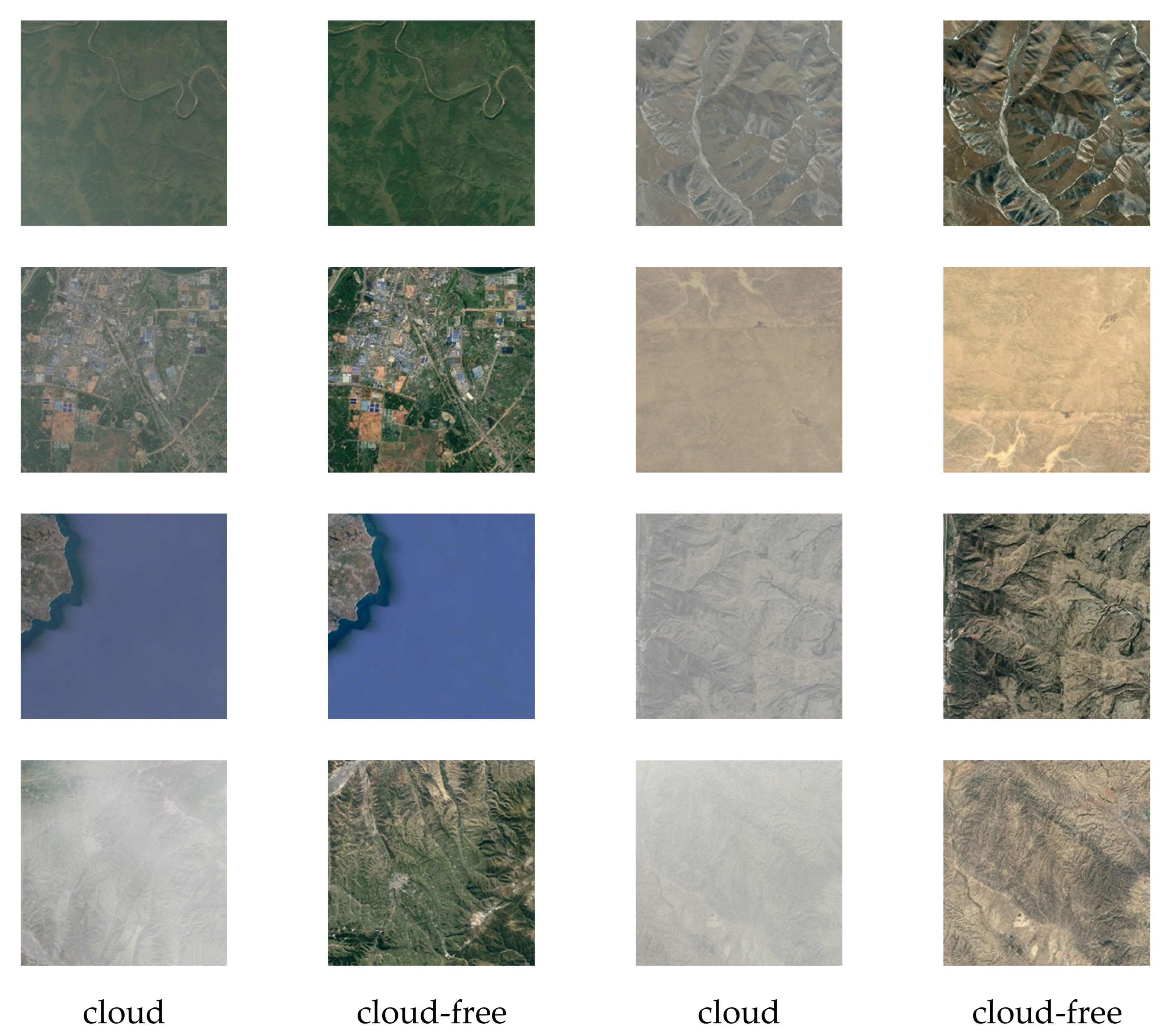
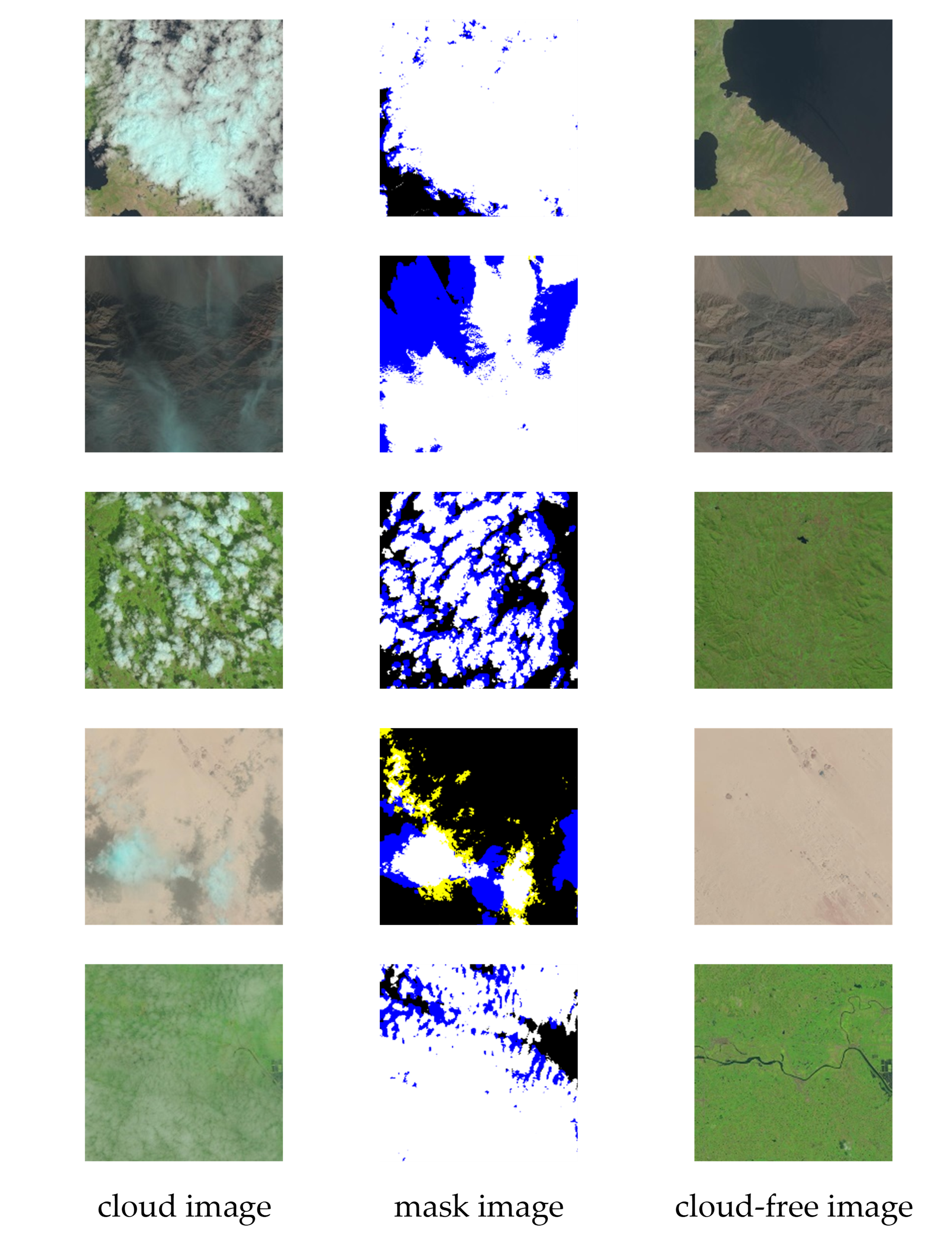
Firstly, we present two subsets of a benchmark dataset named RICE (Remote Sensing Image Cloud Removing): RICE-I and RICE-II, which comprise 500 pairs of corresponding cloudy and cloud-free images and additional corresponding masks for comprehensive algorithm evaluation, as shown in Figure 1 and Figure 2.
Secondly, we propose a baseline model with an integrated convolutional attention mechanism specifically designed for the RICE dataset. This mechanism allows the network to better understand the spatial structure, local details, and inter-channel correlations in cloud removal, effectively addressing the varied distribution of clouds observed in remote sensing images.
Lastly, we introduce the use of the Learned Perceptual Image Patch Similarity (LPIPS) metric, which emphasizes perceptual similarity, aligning with the human visual system’s perception, for a more accurate evaluation of the quality of generated cloud-free images.
In summary, our contributions can be logically summarized as follows:
Introduction of the RICE dataset, which includes 1236 pairs of cloudy and cloud-free remote sensing images with corresponding masks, serving as a comprehensive evaluation resource for cloud removal algorithms.
A baseline model incorporating a convolutional attention mechanism, which enhances the network’s ability to comprehend the spatial structure, local details, and inter-channel correlations present in remote sensing images, thereby effectively addressing the diverse distribution of clouds.
Adoption of the LPIPS metric for evaluating the quality of generated cloud-free images, focusing on perceptual similarity to better match human visual perception.
The RICE-I dataset encompasses a comprehensive collection of 500 image pairs from Google Earth. Acquiring the corresponding cloud and cloudless images involves adjusting the display settings to include or exclude the cloud layer. Subsequently, the acquired images are uniformly cropped to a standardized size of 512×512 pixels. In contrast, the RICE-II dataset includes 736 image pairs from Landsat 8 OLI and TIRS products. Similar to the RICE-I dataset, the images in RICE-II are also cropped to ensure consistency, with each image patch measuring 512×512 pixels and devoid of overlapping regions.
Distinct from the RICE-I dataset, the image patches in RICE-II are meticulously labeled into three explicitly defined classes: cloud-free, cloud mask, and cloud. We selected images captured in the same location within 15 days to obtain paired optical datasets with cloudy and clear conditions. This strict temporal constraint ensures that the images within each pair closely correspond to the prevailing atmospheric conditions.
The RICE dataset encompasses extensive ground scenes, showcasing diverse landscapes such as water bodies, urban areas, deserts, barren lands, forests, and grass-lands. This diversity allows for a comprehensive evaluation of algorithms and models for cloud detection and removal tasks, ensuring their robustness across various environmental contexts.
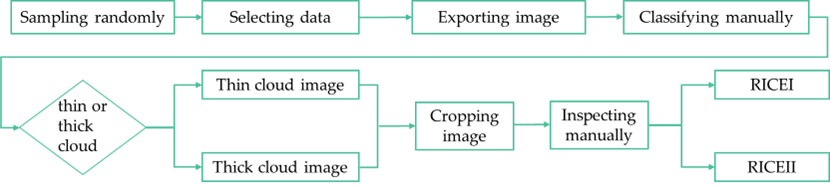
During the process of creating a dataset, we used the cloud-based remote sensing platform Google Earth Engine, and the steps of the dataset generation procedure are described in Figure 3. Acquiring the corresponding cloud and cloudless images involves adjusting the display settings to include or exclude the cloud layer. Subsequently, the acquired images are uniformly cropped to a standardized size of 512×512 pixels.
The RICE dataset can be accessed and downloaded from the following GitHub repository: https://github.com/BUPTLdy/RICE_DATASET. Figure 1 and 2 provide examples of data from RICE-I and RICE-II, respectively, illustrating the dataset’s characteristics.
In order to comprehensively assess the effectiveness of algorithm models in cloud detection and removal tasks, several performance metrics are utilized. These metrics encompass both objective quantitative measures and subjective visual evaluations, providing a holistic assessment of the generated images. The subjective evaluation offers valuable insights into the perceptual quality of the generated images, capturing aspects that may not be entirely captured by quantitative metrics alone.
Two widely used methods for evaluating the quality of images are the structural similarity index measurement (SSIM) and the peak signal-to-noise ratio (PSNR) [30]. The SSIM metric measures the similarity between the generated image and the ground truth image, taking into account factors such as luminance, contrast, and structural information. It is a quantitative method used to evaluate the performance of algorithms. On the other hand, the PSNR metric quantifies the level of noise or distortion present in the generated image by comparing it to the original high-quality image.
SSIM is a well-established metric used to quantitatively assess the degree of structural similarity between a generated image and its corresponding ground truth image. SSIM considers various visual attributes, including luminance, contrast, and structural similarities, to evaluate the resemblance between the two images. A higher SSIM value indicates a more significant similarity between the generated image and the ground truth image, suggesting a higher quality of the generated image.
SSIM operates by emulating the perceptual processes of the human visual system, which is sensitive to local structural changes in images arising from variations in brightness, contrast, and structure. By modeling these perceptual aspects, SSIM provides a reliable measure of the visual similarity between two images. The SSIM value is directly proportional to the resemblance between the images, with larger SSIM values indicating higher similarity [31]. The mathematical formulation for computing the SSIM value between two images, denoted as x and y, is crucial for understanding its application in image quality assessment. The SSIM index is calculated on various windows of an image, which can be compared with the corresponding windows of the ground truth image. The mathematical formulation for computing the SSIM value between two images, denoted as x and y, can be expressed as shown in Eq. (1).
\[\label{e1} \operatorname{SSIM}_{(x, y)}=\frac{\left(2 \mu_x \mu_y+C_1\right)}{\left(\mu_x^2+\mu_y^2+C_1\right)} \times \frac{\left(2 \sigma_{x y}+C_2\right)}{\left(\sigma_x^2+\sigma_y^2+C_2\right)},\tag{1}\] where \(\mu\) is the average of the image and \(\sigma\) is the variances of image, \(\sigma\)2 represents covariance, C1 and C2 are constants for stabilizing the division with a weak denominator. These constants are typically set to small values, and their role is to prevent in-stability when the denominator is close to zero. The SSIM index is a decimal value between -1 and 1, where 1 indicates perfect similarity. This detailed explanation of SSIM, along with its mathematical formulation, provides a clear understanding of how image quality is evaluated in our study.
PSNR is a standard metric in image processing that measures the fidelity of a generated image in comparison to an original ground truth image, by quantifying the ratio of the maximum possible pixel intensity to the mean squared error (MSE) between the two images. A higher PSNR value suggests that the generated image retains a higher fidelity to the original, with lower levels of noise and distortion [32]. While it is a helpful indicator of image reconstruction quality, it may not fully capture all aspects of human visual perception, such as texture and structural integrity. The PSNR can be calculated using Eq. (2).
\[\label{e2} \operatorname{PSNR}=10 \log _{10}\left(\frac{\mathrm{MAX}_I^2}{\mathrm{MSE}}\right),\tag{2}\] where \({{\text{MAX}}_I^2}\) represents the maximum pixel value of the image and MSE is the mean square error.
In addition to the commonly employed metrics such as SSIM and PSNR, the Learned Perceptual Image Patch Similarity (LPIPS) [33] metric has emerged as a significant perceptual measure for assessing the similarity between patches of images. LPIPS considers human perception principles, enabling a more comprehensive evaluation of image quality. By examining the visual similarity between patches, LPIPS captures low-level features, such as color and texture, and high-level semantic information.
By examining the visual similarity between patches, LPIPS captures low-level features, such as color and texture, and high-level semantic information, which is shown in Eq. (3).
\[\label{e3} \operatorname{LPIPS}(x, y)=\sum_l \frac{1}{H_l W_l} \sum_{h, w}\left\|\phi_l(x)_{h, w}-\phi_l(y)_{h, w}\right\|_2^2,\tag{3}\] where \(x\) and \(y\) are the patches from the generated and ground truth images, respectively; \({{H_l}}\) and \({{W_l}}\) denote the height and width of the feature maps at layer \(l\); \({{\phi _l}{{(x)}_{h,w}}}\) represents the feature vector at position \((h,w)\) in the feature maps extracted from layer \(l\) of the deep network; and \(||.|{|_2}\) is the Euclidean distance. This computation integrates the contributions of multiple layers of a deep network, thereby providing a robust and nuanced measure of image quality that takes into account a wide range of visual attributes.
LPIPS quantifies the similarity between two images based on human perception. A smaller LPIPS value indicates higher perceptual similarity between the images. Moreover, human observers possess the ability to discern differences in image details. Given the simplicity of the algorithms employed in image quality assessment and the complexity inherent in real-world image structures, subjective visual analysis can provide an intuitive and comprehensive understanding of detail comparison and equip-ment performance [34].
The primary aim of this study is to put forth a CNN framework explicitly designed for cloud removal in remote sensing imagery. This undertaking involves the conversion of an image that has been adversely affected by the presence of clouds, referred to as the cloud-contaminated image, into a pristine cloud-free image, referred to as, through the effective utilization of deep learning methodologies. By employing the advanced capa-bilities of CNNs, this research seeks to address the challenge of cloud interference in remote sensing data, thereby enhancing the quality and utility of the resultant imagery for various applications.
The input to the CNN model is a cloud-contaminated image x, acquired from remote sensing sensors. The image is represented as a two-dimensional matrix, where each element corresponds to a pixel value. The dimensions of the input image vary based on the resolution of the remote sensing system. Let \(x \in {R^ \wedge }(H \times W \times C)\) represent the input image, where H W, and C denote the height, width, and number of channels, respectively.
The task can be defined as learning a mapping function F: \(x \in {R^ \wedge }(H \times W \times C) \to y \in {R^ \wedge }(H \times W \times C)\) that takes a cloud-contaminated image x as input and produces a cloud-free image y as output. The objective is to train the CNN model to accurately learn this mapping function, enabling it to effectively remove clouds from remote sensing imagery.
Dong et al. [35,36] developed SRCNN, a deep CNN depicted in Figure 4, which directly converts low-resolution images to high-resolution images. It uses bicubic interpolation to upscale LR images [32] and employs three convolutional layers with Leaky ReLU activation. The first layer has 64 filters applied to the upscaled LR blocks [37], the second with 64 filters aids in nonlinear mapping, and the third with three filters reconstructs the HR image from patches [38].
In this article, the SRCNN model is applied to two distinct datasets with the intention of removing cloud interference from satellite images. For the RICE-I dataset, the model processes images that are marred by clouds, aiming to output clean, cloud-free images. The SRCNN is trained to detect and eliminate the cloud distortions, revealing the obscured details of the earth’s surface. For the RICE-II dataset, the challenge is augmented by providing the SRCNN model with inputs that combine cloud-contaminated images with a cloud mask appended as an extra channel. This cloud mask offers valuable information about the cloud coverage, assisting the model in more accurately predicting and generating cloud-free images. In both instances, the goal is to use the SRCNN to transform obscured satellite images into usable data, beneficial for various downstream tasks such as climate analysis, land usage mapping, and disaster management. Consequently, the input of the first convolutional layer of SRCNN is conv(3,f1,n1,6), where f1 represents the filter size and n1 represents the number of filters. The remaining parameters of the SRCNN model remain unchanged. The same processing approach is applied to the other methods in this article.
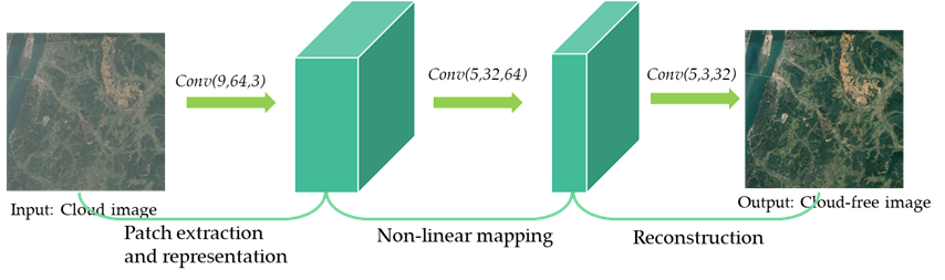
Figure 5 illustrates the architecture of the Very Deep Super-Resolution (VDSR) method, which consists of twenty convolutional neural network (CNN) layers and nineteen Rectified Linear Unit (ReLU) layers [38]. For this approach, an unsampled image is taken as the input, and a residual image is generated as the regression output [39]. A High-Resolution image can be obtained by combining the interpolated image with the residual image [40].
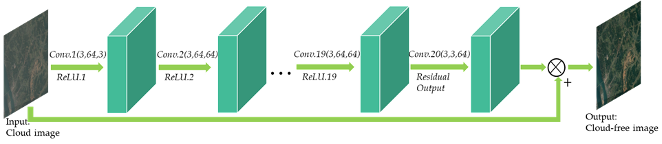
In the context of cloud removal in remote sensing imagery, the VDSR model is employed to address this task. The VDSR model takes a cloud-contaminated image as its input and aims to produce a cloud-free image as the desired output. The primary objective of the VDSR algorithm is to effectively eliminate the cloud artifacts present in the input image while improving its visual quality. This is accomplished through the model’s ability to learn and exploit the residual details between the cloud-contaminated input and the desired cloud-free output. By leveraging the deep architecture of VDSR, the model can capture and comprehend intricate spatial dependencies within the image data, thus facilitating the generation of high-quality, cloud-free images. Moreover, integrating the interpolated image with the residual image further enhances the overall output, leading to visually appealing and cloud-free images suitable for various remote sensing applications.
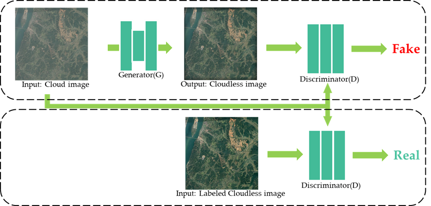
Generative Adversarial Networks (GANs) have gained popularity for improving super-resolution image generation, as evidenced by various studies [41]. GANs consist of a generator (G) and a discriminator (D), depicted in Figure 6, and require matching input and output images for training. In this research, GANs are employed for cloud removal from images; the generator takes a cloud-contaminated image as input, while the discriminator evaluates the generator’s cloud-free output against the real, labeled cloud-free image to verify its authenticity.
Two popular GAN-based approaches used for cloud removal are Pix2pix and SRGAN [42]. SRGAN’s generator adopts a ResNet structure, while its discriminator follows the VGG-19 network structure [43]. On the other hand, Pix2pix utilizes a well-designed U-Net as the generator and a PatchGAN structure as the discriminator [44].
By employing GANs for cloud removal, the models aim to generate realistic and visually appealing cloud-free images by learning the underlying patterns and structures from the labeled cloud-free images. The adversarial training process between the generator and discriminator helps refine the generator’s performance, improving cloud removal results.
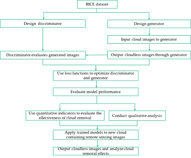
The cloud removal process from remote sensing imagery using GANs commences with assembling and labeling a dataset to distinguish between cloudy and clear images. These images are then preprocessed for network compatibility. A generator network is tasked with creating cloud-free images from the cloudy inputs, while a discriminator network evaluates the authenticity of the generated images. Both networks are trained and optimized through a loss function. The trained model is then assessed using an independent test set for both quantitative metrics and qualitative analysis. Finally, the refined model is applied to new images to produce declouded outputs which are analyzed to evaluate the cloud removal performance (see Figure 7 ).
In the context of cloud removal techniques in remote sensing imagery, the Convolutional Block Attention Module (CBAM) emerges as an innovative approach that enhances the model’s ability to identify and concentrate on cloud regions, extract relevant cloud attributes dynamically, and effectively mitigate extraneous factors unrelated to clouds. By incorporating CBAM, the model’s cloud-centric capabilities can be augmented, improving performance in removing clouds from remote sensing images. This research aims to enhance the model’s adaptability by leveraging CBAM to capture cloud-related features while simultaneously suppressing the impact of non-cloud disturbances or interferences.
The CBAM incorporates a convolutional attention mechanism that assigns higher attention weights to cloud regions, enabling the model to concentrate on clouds effectively. This mechanism enhances the model’s understanding of cloud location, shape, and distribution, thereby improving its ability to accurately detect and segment cloud regions. The convolutional attention mechanism of CBAM allows the model to learn features from cloud regions adaptively. This capability enables the model to extract better cloud texture, shape, color, and other characteristics. Consequently, the model becomes more proficient in distinguishing between cloud layers and surface information, even in complex remotesensing images. Suppressing non-cloud interference: By incorporating the attention mechanism, the model can selectively suppress interfering features in non-cloud regions. This capability helps the model to differentiate clouds from other objects more effectively, reducing false detections and missegmentation.
The CBAM encompasses two pivotal constituents: the channel attention module and the spatial attention module []. The structural configuration of the CBAM is depicted in Figure 8 [46]. Initially, the feature map undergoes processing in the channel attention module, resulting in the generation of an attention map tailored to the specific channels. Subsequently, the input feature map is subjected to elementwise multiplication with the channel attention map, yielding a novel attention map. Analogously, the obtained attention map serves as the input feature map for the spatial attention module, culminating in the production of the final feature map [47]. By integrating the CBAM module towards the concluding stages of convolutional neural network (CNN) architectures, the neural network becomes adept at concentrating on pertinent features while disregarding inconsequential ones, leading to discernible enhancements in experimental accuracy [48].

In this paper, the network structures of various methods are shown in Table 1. The notation conv(k,c1,c2,’act’)*n represents a sequence of n consecutive convolutional layers, where the kernel size is k, the input channels are c1, the output channels are c2, and ’act’ denotes the activation function. For dataset RICE-I, the input consists of cloud-free remote sensing images, and the input channels of the first convolutional layer are c1=3. On the other hand, for dataset RICE-II, the input includes cloud-free remote sensing images and masks indicating the locations of clouds, so the input channels of the first convolutional layer are c1=6.
| Methods | Network Structure | |
|---|---|---|
| SRCNN | conv(9, 3, 64, ’ReLU’) | |
| – | conv(5, 64, 32, ’ReLU’) | |
| – | conv(5, 32, 3, None) | |
| – | VDSR | conv(3,3,64, ReLU) |
| – | conv(3, 64, 64, ’ReLU’)*9 | – |
| – | conv(3, 64, 3, None) | |
| – | Generator: | Discriminator: |
| Pix2pix | conv(3, 3, 64, ’ReLU’) | conv(4, 3, 64, ’Leaky_ReLU’) |
| – | conv(3, 64, 128, ’ReLU’) | conv(4, 64, 128, ’Leaky_ReLU’) |
| – | conv(3, 128, 256, ’ReLU’) | conv(4, 128, 256, ’Leaky_ReLU’) |
| – | conv(3, 256, 256, ’ReLU’)*4 | conv(4, 256, 512, ’Leaky_ReLU’) |
| – | conv(3, 256, 128, ’ReLU’) | conv(4, 512, 1, None) |
| – | conv(3, 128, 64, ’ReLU’) | – |
| – | conv(3, 64, 3, ’tanh’) | – |
| – | Generator: | Discriminator: |
| – | conv(9,3,64,ReLU) | conv(3,3,64,Leaky_ReLU) |
| – | conv(3, 64, 64, ReLU)*7 | conv(3, 64, 64, Leaky_ReLU) |
| – | conv(3, 64, 3, None) | conv(3, 64, 128, Leaky_ReLU) |
| SRGAN | – | conv(3, 128, 128, ’Leaky_ReLU’) |
| – | – | conv(3, 128, 256, ’Leaky_ReLU’) |
| – | – | conv(3, 256, 256, ’Leaky_ReLU’) |
| – | – | conv(3, 256, 512, ’Leaky_ReLU’) |
| – | – | conv(3, 512, 512, ’Leaky_ReLU’) |
| – | – | conv(1, 512, 1, None) |
To ensure robust evaluation, the dataset used in this study was partitioned into five folds for crossvalidation. The Adam optimizer was selected as the optimization algorithm to train the network, employing a learning rate of 0.00001. To counteract potential overfitting, we incorporated weight decay regularization with a coefficient of 0.0001. The batch size was determined to be 64, taking into consideration both computational resources and empirical performance analysis. Throughout the training process, the model underwent 50 epochs, with early stopping serving as the termination criterion. Specifically, training would cease if the validation loss failed to exhibit improvement for a consecutive span of 10 epochs. Additionally, a learning rate reduction strategy was adopted, wherein the learning rate was reduced by a factor of 0.1 if the validation loss stagnated for five consecutive epochs.
The default configuration of LPIPS incorporates several essential components. Firstly, it employs the VGG-16 architecture to extract features from images, specifically utilizing intermediate layers within the VGG-16 network. Subsequently, LPIPS calculates the perceptual distance by quantifying the Euclidean distance between feature maps. Additionally, spatial pooling is applied to aggregate the feature maps in LPIPS. Moreover, LPIPS incorporates feature normalization techniques to ensure scale-invariant and consistent distance measurements.
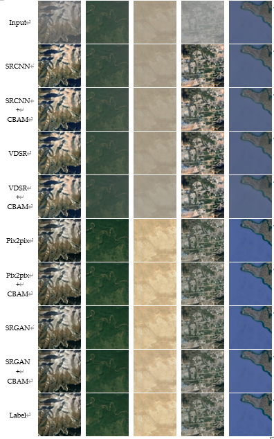
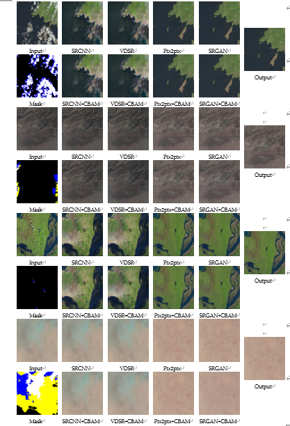
The cloud removal outcomes obtained from the RICE-I dataset are visually depicted in Figure 9. The topmost row of the figure exhibits the input images that contain clouds, while the bottom row showcases the corresponding ground truth cloud-free images. The intermediate rows in the figure present the cloud removal results obtained through the application of baseline methods. Similarly, Figure 10 demonstrates the cloud removal results obtained from the RICE-II dataset. The leftmost column of Figure 10 represents the input images containing clouds, accompanied by their corresponding mask images, while the rightmost column displays the ground truth cloud-free images. The remaining columns of the figure illustrate the cloud removal results generated by the baseline methods.
The experimental findings are presented in Table 2, which provides a comprehensive overview of the evaluation metrics employed in this study. The SSIM is utilized to measure the similarity between two images, with values ranging from 0 to 1. A higher SSIM value indicates a greater resemblance between the two images in terms of their structure, brightness, and contrast. Specifically, an SSIM value of 1 denotes complete identity between the two images. The PSNR is expressed in decibels (dB) and typically ranges from non-negative numbers. A higher PSNR value suggests a smaller disparity between the two images, reflecting improved image fidelity. Furthermore, the LPIPS metric also employs non-negative values, with a lower LPIPS value indicating a higher degree of perceptual similarity between the two images. An LPIPS value of 0 signifies complete perceptual equivalence between the images.
| Methods | RICE-I/SSIM | RICE-I/PSNR | RICE-I/ LPIPS | RICE-II/SSIM | RICE-II/PSNR | RICE-II/ LPIPS |
| SRCNN | 0.857 | 28.798 | 0.157 | 0.702 | 28.476 | 0.137 |
| SRCNN + CBAM | 0.884 | 28.877 | 0.149 | 0.789 | 28.582 | 0.126 |
| VDSR | 0.873 | 28.911 | 0.106 | 0.749 | 28.546 | 0.105 |
| VDSR + CBAM | 0.889 | 28.981 | 0.104 | 0.773 | 28.681 | 0.091 |
| Pix2pix | 0.912 | 29.106 | 0.060 | 0.914 | 32.075 | 0.046 |
| Pix2pix + CBAM | 0.913 | 30.612 | 0.045 | 0.916 | 33.749 | 0.038 |
| SRGAN | 0.902 | 29.039 | 0.056 | 0.915 | 33.244 | 0.055 |
| SRGAN + CBAM | 0.914 | 31.923 | 0.085 | 0.911 | 29.631 | 0.067 |
This study addresses the prominent issue of cloud removal in remote sensing imagery, an essential preprocessing step for accurate image analysis. While deep learning has exhibited notable advancements in various remote sensing tasks, the need for suitable training datasets for neural networks has hindered its application to cloud removal. We introduce the RICE dataset to overcome this limitation and propose baseline models incorporating a convolutional attention mechanism. Our proposed models harness the power of the convolutional attention mechanism to enhance the network’s comprehension of spatial structures, local details, and interchannel correlations within remote sensing images. This empowers the models to effectively handle diverse cloud distributions and improve the precision of cloud removal.
Moreover, we introduce the LPIPS metric as an evaluation criterion to assess the fidelity of generated cloud-free images. This metric emphasizes perceptual similarity, providing a more comprehensive image quality assessment. By presenting the RICE dataset and evaluating the fidelity of generated images using the LPIPS metric, this research contributes to advancing cloud removal techniques in remote sensing. The availability of the RICE dataset not only facilitates further research in this area but also enables the development of more robust and accurate cloud removal algorithms.
Overall, our work demonstrates the potential of deep learning in addressing the challenges of cloud removal in remote sensing imagery. Furthermore, it provides a comprehensive evaluation framework for assessing the quality of generated cloud-free images. The findings presented in this study will inspire future research endeavors in this field and contribute to the continual improvement of remote sensing image analysis techniques.
The experimental data used to support the findings of this study are available from the corresponding author upon request.
The authors declared that they have no conflicts of interest regarding this work.