
A \(k\)-ranking (or simply “ranking”) on a graph \(G\) is defined to be a function \(f: V(G) \rightarrow \left\{ 1, 2, \ldots, k \right\}\) with the following restriction: if \(f(u)=f(v)\) for any \(u, v \in V(G)\), then on every \(uv\) path in \(G\), there exists a vertex \(w\) with \(f(w) > f(u)\). This vertex labeling problem has generated great interest because of its applications to Cholesky factorization of matrices in parallel [2-4], VLSI layout [5,6] and scheduling steps in manufacturing systems [7,8].
The focus of much of the literature on rankings has been on minimizing \(k\). That is, given a graph \(G\), the goal is to determine the minimum number of labels required to produce a valid ranking on \(G\). The minimum number of labels required to produce a ranking on a graph \(G\) is called the rank number of \(G\), and is denoted \(\chi_r(G)\). Note that on a graph \(G\), a ranking with \(\chi_r(G)\) labels is a ranking with smallest \(l_{\infty}\) or max norm.
However, in [9], Jamison and Narayan compare the rank number of \(G\) with the lowest possible sum, or \(l_1\) norm, of all rankings on \(G\). In particular, they show that for paths and cycles, \(l_1\)-optimal rankings are also max optimal.
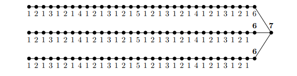
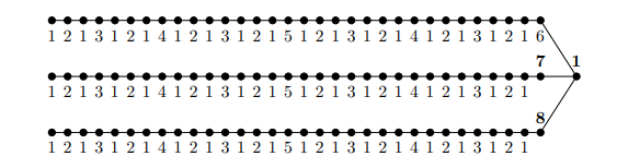
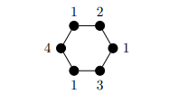
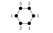
The results in [9] give rise to the question of how changing the value of \(p\) affects \(l_p\) optimality of a ranking. While most commonly known applications of \(l_p\) norms with finite \(p\) use \(p \in \{1, 2 \}\), some applications have used finite \(p\) with \(p \notin \{1, 2\}\). Some examples include machine learning [10,11], compressed sensing [12], image deconvolution [13], and two-dimensional phase unwrapping [14]. Specific to \(k\)-rankings on graphs, a graph may have distinct \(l_p\)-optimal rankings for two different values of \(p\), even if both values of \(p\) satisfy \(1<p<\infty\). For example, Figures 1–2 display a graph whose sets of \(l_2\)– and \(l_3\)-optimal rankings are disjoint.
In [1] we showed that for any \(p \geq 0\) and any non-negative integer \(c\), we can construct a graph with \(c\) cycles such that the sets of \(l_p\)-optimal and \(l_{\infty}\)-optimal rankings are disjoint. In this paper, we show that there are families of graphs including paths, cycles, and complete multipartite graphs such any \(l_p\)-optimal ranking is also \(l_{\infty}\) optimal for any \(p\) with \(0 \leq p < \infty\).
We will use the notion of minimality of a ranking throughout the paper.
Definition 1. A ranking is minimal if decreasing any label to a smaller label violates the definition of a ranking.
The concept of a reduction, defined by Ghoshal, Laskar and Pillone will also be used throughout.
Definition 2. [15] For a graph \(G\) and a set \(S \subseteq V=V(G)\), the reduction of \(G\) with respect to \(S\), denoted \(G_S^{\flat}\), is the subgraph of \(G\) induced by \(V-S\), with an additional edge \(uv \in E(G_S^{\flat})\) for each \(u, v \in V-S\) if and only if there exists a \(uv\) path in \(G\) with all internal vertices belonging to \(S\).
For a ranking \(f\) on a graph \(G\), define \(S_i(f)\) by \(S_i(f) = \left\{ v \in G ~| ~ f(v) = i \right\}.\) In general, a reduction can be applied with respect to any set \(S \subseteq V(G)\). However, for the purposes of our paper, we primarily consider the case where \(S=S_1(f)\) for some ranking \(f\) on \(G\). When the set \(S\) is understood, we denote \(G_{S}^{\flat}\) by \(G^{\flat}\).
Because for our purposes the reduction often depends on the ranking we consider, we also define a new ranking associated with \(G^{\flat}\) as follows. Let \(G\) be a graph, and \(f\) a ranking on \(G\). For any subgraph \(H\) of \(G\), we define a ranking \(f_H\) by setting \(f_H(v)=f(v)\) for all \(v\in V(H)\). If \(H=G^{\flat}_{S_1(f)}\), set \(f_H(v)=f(v)-1\) for all \(v\in V(H)\). Note that \(f_H\) is a ranking on \(H\) and is called a reduction ranking.
We can define a similar labeling if \(S \neq S_1(f)\) by setting \(f_H(v)=f(v)\) for all \(v \in V(H)\) where \(H\) is the reduction. However, the resulting labeling is not guaranteed to be a ranking. In this case we call the labeling a reduction labeling. An expansion of \(G\) is a graph \(G^{\sharp}\) such that \(\left( G^{\sharp} \right)^{\flat}_S = G\) for some \(S \subseteq V( G^{\sharp})\).
Finally, we note the following result from [15].
Lemma 1. [15] If \(f\) is a minimal ranking on \(G\), then the reduction ranking \(f_{G_{S_1(f)}^{\flat}}\) is a minimal ranking on \(G^{\flat}_{S_1(f)}\).
For a graph \(G\) with ranking \(f\), and \(1 \leq p < \infty\), the \(l_p\) norm of \(f\) is given by the \(l_p\) norm of the labels of \(f\): \[\label{eq:lp} \left\| f \right\|_p = \left( \sum_{v \in V(G)} \left[ f(v) \right]^p \right)^{1/p}.\tag{1}\] If \(p=1\), this describes the norm considered in [9], and \(p=2\) corresponds to the standard Euclidean norm. The standard existing norm in the literature on graph rankings is the supremum or max, or \(l_{\infty}\) norm: \[\left\| f \right\|_{\infty} = \max_{v \in V(G)} f(v).\] For \(0<p<1\), \(||\cdot||_p\) is defined as in (1), but fails to be a norm. The case \(p=0\) is considered separately in Section 5.
We refer to a ranking \(f\) on \(G\) that achieves \(||f||_{\infty} = \chi_r(G)\) as a max optimal ranking. Given a graph \(G\), a ranking \(f\) and non-negative real number \(p\), we say that \(f\) is \(l_p\) optimal if \[\left\| f \right\|_{p} = \min \left\{ \left\| g \right\|_p \mid g \mbox{ is a ranking on } G\right\}.\] We define an analog of the rank number to \(l_p\) optimality.
Definition 3. For a graph \(G\) and non-negative real number \(p\), the \(l_p\)-rank number of \(G\), \(\chi_r^p(G)\) is \(\left\| f \right\|_{p}\) where \(f\) is an \(l_p\)-optimal ranking on \(G\).
For any non-negative real number \(p\), if \(f\) is not minimal then we can reduce one of the labels to produce a ranking \(\tilde{f}\) with \(||\tilde{f}||_p < ||f||_p\).
Observation 1. For \(p \in (0, \infty)\), if \(f\) is an \(l_p\)-optimal ranking on a graph \(G\), then \(f\) is minimal.
Note that observation 1 does not hold if \(p=0\) or \(p=\infty\).
Proposition 1. Let \(G\) be a graph, and let \(H\) be any subgraph of \(G\). Then for any non-negative real number \(p\), \(\chi_{r}^{p}(H) \leq \chi_r^p(G).\)
Proof. Suppose \(g\) is an \(l_p\)-optimal ranking on \(G\). Then \(g_H\) is a ranking and \[\left(\chi_r^p(H)\right)^p\leq ||g_H||_p^p = \sum_{v\in H} g(v)^p \leq \sum_{v\in G} g(v)^p = ||g||_p^p = \left( \chi_r^p(G) \right)^p.\] ◻
Lemma 2. Let \(f\) be any \(l_p\)-optimal ranking on a graph \(G\). Also, let \(\mathcal{S}\) be a non-empty subset of \(S_1(f)\) and let \(G^{\flat} = G^{\flat}_{\mathcal{S}}\). Then \(\chi_r^p(G^{\flat}) < \chi_r^p(G)\).
Proof. Note that \(f_{G^{\flat}}\) is a ranking on \(G^{\flat}\) because the only vertices removed have label \(1\). By the definition of a reduction ranking, \(||f_{G^{\flat}}||_p < ||f||_p.\) Hence, \(\chi_r^p(G^{\flat}) < \chi_r^p(G).\) ◻
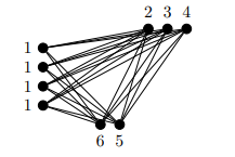
We note here that a graph may have different \(l_p\)-optimal rankings depending on the value of \(p\), even when \(p\) is restricted to \(1<p<\infty\), as illustrated by the example shown in Figures 1–2. Figure 1 shows a ranking \(f\) that is \(l_3\) optimal but not \(l_2\) optimal, while Figure 2 shows a ranking \(g\) of the same graph that is \(l_2\) optimal but not \(l_3\) optimal. Since \(f(v) = g(v)\) for all \(v \in V\) except for the vertex of degree \(3\) and vertices \(u\) and \(w\) with \(g(u)=7\) and \(g(w)=8\), we can compute that \(\|g\|_3^3 – \|f \|_3^3 =81 > 0\), but \(\|f\|_2^2 – \|g\|_2^2 = 7 > 0\).
In Sections 2 and 3, we show any \(l_p\)-optimal ranking on a path or cycle where \(p > 0\) is also max optimal, but that the converse does not hold. In Section 4 we show that on a complete multipartite graph a ranking is \(l_p\) optimal if and only if it is max optimal. Throughout Sections 2 – 4 we assume \(0 < p < \infty\) unless otherwise stated. Finally, in Section 5, we show that if \(p=0\), then \(l_p\) optimality does not imply max optimality in paths and cycles, but that the result for complete multipartite graphs holds with the added assumption of minimality. We conclude with some open questions in Section 6.
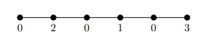
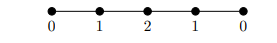
Let \(P_n\) denote a path on \(n\) vertices, \(v_1, v_2, \ldots, v_n\). We can construct a ranking \(f\) for \(P_n\) in a greedy fashion by starting with \(v_1\), and defining \(f(v_i)\) to be the lowest label possible without violating the definition of ranking, producing the standard ranking of a path as shown in Figure 3.
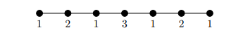
Bodlaender et al. [2] showed that \(\chi_r(P_n) = \left\lfloor \log_2 n \right\rfloor +1\) and that the standard ranking \(f\) is a max optimal ranking on \(P_n\). Note that the standard ranking \(f\) on \(P_n\) can also be defined by letting \(f(v_i)=r+1\) where \(r\) is the highest power of 2 that divides \(i\).
In this section, we show that any \(l_p\)-optimal ranking on \(P_n\) is also a max optimal ranking. Throughout the section, given a ranking \(f\) on \(G=P_n\), we use the notation \(f^\flat\) to refer to the reduction ranking on \(G^{\flat}_{S}\) where \(S=S_1(f)\). Similarly, given a ranking \(f\) on a path \(P_{\lfloor n/2 \rfloor}\), we use the notation \(f^\sharp\) to refer to the expansion ranking on \(P_n\) formed by adding 1 to all existing labels, inserting a vertex labeled \(1\) between each consecutive pair of vertices in \(P_{\lfloor n/2 \rfloor}\) and to the front of the path, and, if \(n\) is odd, adding one more vertex labeled \(1\) to the end of the path.
Observation 2. Suppose \(f\) is an \(l_p\)-optimal ranking on \(P_n\), and \(g\) an \(l_p\)-optimal ranking on \(P_{n+1}\). Then \(||f||_p < ||g||_p\).
Lemma 3. If \(f\) is an \(l_p\)-optimal ranking on \(P_n\), then \(\left| S_1(f) \right|= \lceil n/2 \rceil\).
Proof. Since \(f\) is a ranking, if \(uv \in E(G)\), then \(f(u) \neq f(v)\). Therefore, \(\left| S_1(f) \right| \leq \lceil n/2 \rceil\). For the other direction, suppose \(g\) is a ranking on \(P_n\) with \(|S_1(g)| < \lceil n/2 \rceil\). Let \(h\) be an \(l_p\)-optimal ranking on \(P_{\lfloor n/2 \rfloor}\). Then, applying Observation 2 to the second step, \[\begin{aligned} ||g||_p^p &= 1^p \left| S_1 (g) \right| + \sum_{v\notin S_1(g)} \left( g^\flat(v) + 1\right)^p \\ &> \left| S_1(g) \right| +\left( \lceil n/2 \rceil – |S_1(g)| \right) 2^p +\sum_{v \in V(P_{\lfloor n/2 \rfloor})} \left( h(v)+1 \right)^p \\ &> \lceil n/2 \rceil +\sum_{v \in V(P_{\lfloor n/2 \rfloor})} \left( h(v)+1 \right)^p = \left\| h^{\sharp} \right\|_p^p \end{aligned}\] Therefore \(g\) is not \(l_p\) optimal since \(h^{\sharp}\) is a ranking on \(P_n\). Hence, if \(f\) is an \(l_p\)-optimal ranking, \(\left| S_1(f) \right|= \lceil n/2 \rceil.\) ◻
Lemma 4. A ranking \(f\) on \(P_n\) is \(l_p\) optimal if and only if \(f^{\flat}\) is an \(l_p\)-optimal ranking on \(P_{\left\lfloor n/2 \right\rfloor}\).
Proof. Let \(f\) be an \(l_p\)-optimal ranking on \(P_n\). We know that \(||f||_p^p = \left\lceil n/2 \right\rceil + \sum_{v \notin S_1(f)} \left(f^\flat(v)+1\right)^p\) by Lemma 3. If \(f^{\flat}\) is not an \(l_p\)-optimal ranking on \(P_{\left\lfloor n/2 \right\rfloor}\), then there exists an \(l_p\)-optimal ranking \(g\) on \(P_{\left\lfloor n/2 \right\rfloor}\), and an expansion \(g^{\sharp}\) such that \[\begin{aligned} ||g^{\sharp}||_p^p &= \lceil n/2 \rceil + \sum_{v \in V(P_{\left\lfloor n/2 \right\rfloor})} \left( g(v) +1 \right)^p \\ &< \lceil n/2 \rceil +\sum_{v\notin S_1(f)} \left( f^{\flat}(v) +1 \right)^p = ||f||_p^p, \end{aligned}\] contradicting the optimality of \(f\). Hence, \(f^{\flat}\) is an \(l_p\)-optimal ranking on \(P_{\left\lfloor n/2 \right\rfloor}\).
Conversely, suppose that \(f^{\flat}\) is an \(l_p\)-optimal ranking on \(P_{\left\lfloor n/2 \right\rfloor}\). Then by construction, \(f\) is a ranking on \(P_n\) with \(\left| S_1(f) \right|= \lceil n/2 \rceil\). If \(f\) is not \(l_p\) optimal, then there exists an \(l_p\)-optimal ranking \(g\) on \(P_n\). By Lemma 3, \(\left| S_1(g) \right|= \lceil n/2 \rceil\). But then the reduction ranking \(g^\flat\) on \(P_{\lfloor n/2 \rfloor}\) has \(||g^\flat||_p < ||f^\flat||_p\), contradicting the optimality of \(f^\flat\). ◻
From Lemma 4, we get the following corollary.
Corollary 1. Let \(f\) be an \(l_p\)-optimal ranking on \(P_n\). Then for any \(j\) with \(2 \leq j \leq \chi_r^p(P_n)\), \[\left| S_j(f) \right| = \left\lceil \frac{n – \sum_{i=1}^{j-1} \left| S_i(f) \right| }{2} \right\rceil.\]
Lemma 5. A ranking \(g\) is a standard ranking on \(P_{\lfloor n/2 \rfloor}\) if and only if \(g^\sharp\) is a standard ranking on \(P_n\).
Proof. The ranking \(g\) is a standard ranking on \(P_{\lfloor n/2 \rfloor}\) if and only if for each \(i\), \(1 \leq i \leq \lfloor n/2 \rfloor\), \(g(v_i) = r+1\) where \(2^r\) is the largest power of 2 that divides \(i\) if and only if (1) \(g^\sharp(v_{2i}) = r+2\) where \(2^{r+1}\) is the highest power of 2 that divides \(2 i\), and (2) \(g^\sharp(v_{2i-1})=1\) for any \(i\). This is true if and only if \(g^\sharp (v_j) = \tilde{r} + 1\) where \(2^{\tilde{r}}\) is the highest power of 2 that divides \(j\) for each \(j\), \(1 \leq j \leq n\). Specifically, for even \(j\), \(\tilde{r}=r+1\) and for odd \(j\), \(\tilde{r} = 0\). ◻
Observation 3. Suppose \(f\) and \(g\) are rankings on a graph \(G\), such that for any positive integer \(i\), \(|S_i(f)| = |S_i(g)|\). Then for any positive integer \(i\), \(|S_i(f_{G^{\flat}_{S_1(f)}})| = |S_i(g_{G^{\flat}_{S_1(g)}})|\). The expansions of \(f\) and \(g\) that label all new vertices with label \(1\) also have the same number of vertices of each label.
Given a path \(P_n\), let \(\mathcal{S}_{j;n}\) denote the set of vertices with label \(j\) under the standard ranking on \(P_n\).
Lemma 6. A ranking \(f\) on \(P_n\) is \(l_p\) optimal if and only if \(|S_j(f)| = |\mathcal{S}_{j;n}|\) for each \(j\geq 1\).
Proof. For \(n=1, 2\) or 3, we can see that the \(l_p\)-optimal rankings are precisely the standard rankings on \(P_n\). Suppose that for any \(n\) up to \(l-1\), a ranking \(f\) on \(P_n\) is \(l_p\) optimal if and only if \(|S_j(f)| = |\mathcal{S}_{j;n}|\) for each \(j\geq 1\).
Using Lemmas 3 and 4, a ranking \(f\) on \(P_l\) is \(l_p\) optimal if and only if \(S_1(f)=\lceil l/2 \rceil\) and \(f^\flat\) is \(l_p\) optimal. Using the inductive hypothesis, \(f^\flat\) is \(l_p\) optimal if and only if \(|S_i(f^{\flat})| = |\mathcal{S}_{i;\lfloor l / 2 \rfloor }|\) for each \(i \geq 1\). For \(i \geq 1\), note that by definition \(|S_i(f^{\flat})| = |S_{i+1}(f)|\), and \(|\mathcal{S}_{i;\lfloor l / 2 \rfloor }| = |\mathcal{S}_{i+1; l }|\) by Lemma 5. Therefore \(f^{\flat}\) is \(l_p\) optimal if and only if \(|S_j(f)| = |\mathcal{S}_{j;l}|\) for each \(j \geq 2\).
Thus, \(f\) is \(l_p\) optimal if and only if \(|S_j(f)| = |\mathcal{S}_{j;l }|\) for each \(j\geq 1\). ◻
Theorem 4. Any \(l_p\)-optimal ranking on \(P_n\) is a max optimal ranking.
Proof. This result is immediate from Lemma 6 and the fact that the standard ranking on \(P_n\) is max optimal. ◻
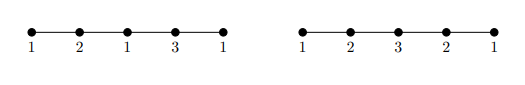
Figure 4 illustrates that the converse of Theorem 4 does not hold, which we now state formally.
Proposition 2. A minimal max optimal ranking on \(P_n\) is not necessarily \(l_p\) optimal.
In [16], Bruoth and Horňák showed the following.
Theorem 5. [16] \(\chi_r(C_n) = \lfloor \log_2(n-1) \rfloor + 2\).
The standard ranking \(f\) on the cycle \(C_n\) is as follows. Starting with any vertex, label the first \(n-1\) vertices \(v_1, v_2, \ldots, v_{n-1}\) greedily in a clockwise direction. Thus, the first \(n-1\) vertices are labeled as the standard ranking on \(P_{n-1}\). Then the final vertex \(v_n\) is labeled \(f(v_n)=\chi_{r}(P_{n-1})+1\). It is well known that the standard ranking \(f\) on a cycle \(C_n\) is a max optimal ranking.
Throughout this section, given a ranking \(f\) on \(G=C_n\), we use \(f^\flat\) to denote the reduction ranking on \(G_S^{\flat}\) where \(S=S_1(f)\). Given a ranking \(g\) on \(C_{\lceil n/2 \rceil}\), we use \(g^\sharp\) to denote the expansion ranking on \(C_n\) obtained as follows: add \(1\) to all labels, then insert \(\lfloor n/2 \rfloor\) vertices labeled \(1\), one between each consecutive pair of vertices in \(C_{\lceil n/2 \rceil}\). If \(n\) is odd, there will be one pair of consecutive vertices in \(C_{\lceil n/2 \rceil}\) that do not receive a new vertex between them. For consistency, we omit the new vertex just before the vertex with highest label in \(C_{\lceil n/2 \rceil}\).
Using similar arguments to the proof of Lemma 3, and applying Lemma 2, we get the following lemma.
Lemma 7. If \(f\) is an \(l_p\)-optimal ranking on \(C_n\), then \(|S_1(f)| = \lfloor \frac{n}{2} \rfloor\).
Lemma 8. A ranking \(f\) on \(C_n\) is \(l_p\) optimal if and only if \(f^\flat\) is an \(l_p\)-optimal ranking on \(C_{\lceil n/2 \rceil}\).
Proof. The proof follows from applying Lemma 4 to arguments similar to those in the proof of Lemma 4. ◻
Corollary 2. If \(f\) is an \(l_p\)-optimal ranking on \(C_n\), then for any \(j\) with \(1 < j \leq \chi_r^p(C_n)\), \[\left|S_j(f)\right| = \left\lfloor \frac{n – \sum^{j-1}_{i=1} |S_i(f)| }{2} \right\rfloor.\]
Proof. This follows from Lemmas 7 and 8. ◻
Lemma 9. A ranking \(g\) on \(C_{\lceil n/2 \rceil}\) is a standard ranking if and only if \(g^\sharp\) is a standard ranking on \(C_n\).
Proof. For \(v_1\) through \(v_{n-1}\), the lemma holds by noting that the standard ranking on a cycle is defined to be the same as the standard ranking on a path for the first \(n-1\) vertices, and Lemma 5.
If \(g^{\sharp}\) is a standard ranking on \(C_n\), then \(g^{\sharp}(v_n) = \chi_r(P_{n-1}) + 1 = \lfloor \log_2(n-1)\rfloor+2\). Then by definition of a reduction ranking, \(g(v_{\lceil n/2 \rceil}) = \chi_r(P_{n-1}) = \left\lfloor \log_2 (n-1) \right\rfloor +1= \left\lfloor \log_2 (\lceil n/2 \rceil – 1) \right\rfloor +2 =\chi_r(P_{\lceil n/2 \rceil -1 })+1\), the standard label. Conversely, if \(g\) is a standard ranking, then \(g(v_{\lceil n/2 \rceil}) = \chi_r(P_{\lceil n/2 \rceil -1 })+1 = \left\lfloor \log_2 (\lceil n/2 \rceil – 1) \right\rfloor +2 = \left\lfloor \log_2 (n-1) \right\rfloor +1 = \chi_r(P_{n-1})\). Then by definition of an expansion, \(g^\sharp(v_n) = \chi_r(P_{n-1}) + 1\), the standard label, completing the proof. ◻
Lemma 10. A ranking \(f\) on \(C_n\) is \(l_p\) optimal if and only if the number of \(v \in V\) with \(f(v)= j\) is the same as the number of vertices in the standard ranking on \(C_n\) with label \(j\).
Proof. The proof follows by applying Lemma 9> and Observation 3 to similar arguments to those in the proof of Lemma 6. ◻
Theorem 6. Any \(l_p\)-optimal ranking on \(C_n\) is also max optimal.
Proof. This is a result of Lemma 10 and the observation that the standard ranking on the cycle is a max optimal ranking. ◻
The converse of Theorem 6 does not hold, as we demonstrate with the following proposition.
Proposition 3. A max optimal ranking on \(C_n\) is not necessarily \(l_p\) optimal.
Proof. Figures 5 and 6 show max optimal rankings \(f\) and \(g\) on \(C_6\), but only \(f\) is \(l_p\) optimal. ◻
We have shown that for paths and cycles, \(l_p\) optimality implies max optimality, but that max optimality does not necessarily imply \(l_p\) optimality. We now show that for any complete multipartite graph \(K_{m_1, m_2, \ldots, m_r}\) with partite sets of order \(m_1 \geq m_2 \geq \cdots \geq m_r\), the set of \(l_p\)-optimal rankings and the set of max optimal rankings are the same.
Lemma 11. If \(f\) is an \(l_p\)-optimal ranking on \(K_{m_1, m_2, \ldots, m_r}\), then under \(f\) every vertex in one of the largest partite sets is labeled \(1\), and all other vertices are labeled using distinct labels.
Proof. Suppose \(f\) is \(l_p\) optimal. Then by observation 1, \(f\) is minimal and thus by [15] \(f\) must label each vertex in one of the partite sets \(W\) the label \(1\), and every other vertex using a distinct label. If \(W\) is not the largest partite set, then a ranking \(g\) can be obtained by labeling every vertex in one of the largest partite sets \(1\), and every other vertex using distinct labels. Now, \(||g||_p<||f||_p\), which implies that \(f\) is not \(l_p\) optimal, a contradiction. ◻
Lemma 12. Let \(f\) be a minimal ranking on \(K_{m_1, m_2, \ldots, m_r}\) such that under \(f\) every vertex in some largest partite set is labeled \(1\), and other vertices are labeled using distinct labels. Then \(f\) is \(l_p\) optimal.
Proof. Suppose \(f\) is a minimal ranking such that every vertex in one of the largest partite sets is labeled \(1\) under \(f\), and other vertices are labeled using distinct labels. Suppose \(g\) is an \(l_p\) optimal ranking. Then, by Lemma 11, \(g\) labels each vertex in one of the largest partite sets \(1\) and other vertices using distinct labels. This means \(||f||_p=||g||_p\), and thus \(f\) is \(l_p\) optimal. ◻
Theorem 7. A ranking on a complete multipartite graph is max optimal if and only if it is \(l_p\) optimal.
Proof. By [15], \(f\) is a minimal ranking if and only if some partite set \(W\) has \(f(w) = 1\) for all \(w \in W\), and all \(v \in V \backslash W\) have unique labels from \(2\) up to \(|V| – |W| + 1\). The minimal ranking \(f\) is a max optimal ranking if and only if the partite set \(W\) has \(|W| = m_1\). Then by Lemmas 11 and 12, \(f\) is max optimal if and only if \(f\) is \(l_p\) optimal. ◻
By noting the a complete graph is a complete multipartite graph \(K_{m_1, m_2, \ldots m_r}\) with \(m_1 = m_2 = \cdots m_r =1\), we get the following immediate corollary.
Corollary 3. A ranking \(f\) on the complete graph \(K_n\) is max optimal if and only if it is \(l_p\) optimal.
Given a sequence of numbers, the \(l_0\) “norm” is defined as the number of non-zero terms in the sequence. For a graph \(G\) with ranking \(f\), \[||f||_0 = \left| \left\{ v \in V(G) \mid f(v) > 0 \right\} \right|.\] The quotation marks indicate that the map fails to satisfy the requirement of homogeneity. Depending on the application [17-20] it is referred to as the zero, counting or Hamming “norm.”
In this section, we use labels \(0\) through \(k-1\) instead of \(1\) through \(k\), because starting with \(1\) leads to \(||f||_0 = |V(G)|\) for every ranking \(f\) on \(G\). We do this on the standard rankings on paths and cycles as well, subtracting \(1\) from each label in the standard ranking. For reductions and expansions, we remove or add vertices with label \(0\) instead of \(1\).
Lemma 13. If \(f\) is an \(l_0\)-optimal ranking on \(P_n\), then \(\left| S_0(f) \right|= \lceil n/2 \rceil\).
Proof. For any ranking \(f\) on a path \(P_n\), \(\left\| f \right\|_0 = n – |S_0(f)|.\) Thus, maximizing the cardinality of \(S_0(f)\) results in an \(l_0\)-optimal ranking. Since \(\left| S_0(f) \right| \leq \lceil n/2 \rceil\) for any ranking \(f\), and the standard ranking \(g\) starting with label \(0\) has \(\left| S_0(g) \right| = \lceil n/2 \rceil\), the result follows. ◻
Corollary 4. \(\chi_{r}^0(P_n) = \lfloor n/2 \rfloor\).
The arank number of a graph \(G\), denoted \(\psi_r(G)\), is given by \(\psi_r(G) = \max\{ ||f||_{\infty} \}\) over any minimal ranking \(f\) on \(G\).
The following theorem shows that neither Theorem 4 nor its converse applies if \(p=0\).
Theorem 8. There exist minimal max optimal rankings on paths that are not \(l_0\) optimal. If \(n=6, 7\) or \(n \geq 10\), then there exists a minimal \(l_0\)-optimal ranking on \(P_n\) that is not max optimal.
Proof. For the first statement, Figure 9 demonstrates a minimal max optimal ranking that is not \(l_0\) optimal. For the second statement, if \(n=6\) or 7, then we have \(\lfloor n/2 \rfloor = 3\); otherwise we have \(\lfloor n/2 \rfloor \geq 5\). In either case, by Lemma 14 we can find a minimal ranking on \(P_{\lfloor n/2 \rfloor}\) that is not max optimal. Choose one such ranking \(f\). Then the ranking \(f^{\sharp}\) is a minimal ranking of \(P_n\): if \(f^\sharp (v) > 0\), then we know it cannot be lowered to a label greater than \(0\) by minimality of \(f\); it cannot be lowered to \(0\) because every vertex not labeled \(0\) is adjacent to a vertex labeled \(0\). Also, \(f^{\sharp}\) is not a max optimal ranking, but is \(l_0\) optimal by Corollary 4 since \(||f||_0 = n – |S_0| = \lfloor n/2 \rfloor.\) ◻
Lemma 15. If \(f\) is an \(l_0\)-optimal ranking on \(C_n\), then \(|S_0(f)| = \lfloor \frac{n}{2} \rfloor\).
Corollary 5. \(\chi_r^0(C_n)= \lceil n/2 \rceil\).
Neither Theorem 6 nor its converse applies to the case \(p=0\), as shown by the following theorem.
Theorem 9. There exist cycles with minimal max optimal rankings that are not \(l_0\) optimal. If \(\psi_r(C_{\lceil n/2 \rceil}) > \chi_r(C_{\lceil n/2 \rceil})\), then \(C_n\) has a minimal ranking \(f\) that is \(l_0\) optimal but not max optimal.
Proof. For the first statement, note that subtracting \(1\) from each of the labels in Figure 6 results in a max optimal ranking that is not \(l_0\) optimal. For the second statement, suppose \(\psi_r(C_{\lceil n/2 \rceil}) > \chi_r(C_{\lceil n/2 \rceil})\). Let \(f\) be a minimal ranking on \(C_{\lceil n/2 \rceil}\) that is not max optimal. Then \(f^{\sharp}\) is a minimal \(l_0\)-optimal ranking of \(C_n\), but is not max optimal. ◻
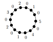
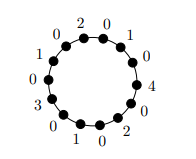
Figure 10 shows a minimal \(l_0\)-optimal ranking on \(C_{14}\) that is not max optimal. Figure 11 shows the standard ranking on \(C_{14}\), which is max optimal.
Finally, we show that unlike paths and cycles, complete multipartite graphs have the same property with regard to \(l_0\) optimality as with \(l_p\) optimality, as long as we require minimality of the \(l_0\)-optimal ranking.
Proposition 4. A ranking \(f\) on a complete multipartite graph is max optimal if and only if it is minimal and \(l_0\) optimal.
Proof. Let \(K_{m_1, m_2, \ldots m_n}\) be a complete multipartite graph with partite sets of order \(m_1 \geq m_2 \geq \cdots \geq m_n\). By [15], and subtracting \(1\) from all labels, \(f\) is a max optimal ranking if and only if a partite set \(W\) with \(|W| = m_1\) has all vertices labeled \(0\), and all \(v \in V \backslash W\) have unique labels from \(1\) up to \(|V| – |W|\).
Let \(g\) be a minimal \(l_0\)-optimal ranking on \(K_{m_1, m_2, \ldots m_n}\). Since \(g\) is minimal, some partite set \(W\) has all vertices labeled \(0\), and all \(v \in V \backslash W\) have unique labels from \(1\) up to \(|V| – |W|\). Then \(||g||_0 = |V| – |W|\). To minimize \(|V|-|W|\), we must have \(|W|=m_1\), and then \(\|g\|_0 = |V| – m_1\). ◻
For paths and cycles, we have shown that \(l_p\) optimality of a ranking implies max optimality for all \(p>0\). For \(p=0\), we have shown that this does not hold. We have also shown that max optimality does not imply \(l_p\) optimality for these graphs. For complete multipartite graphs, however, we showed that the set of \(l_p\)-optimal rankings is the same as the set of max optimal rankings, including in the case \(p=0\) if we restrict \(l_0\)-optimal rankings to be minimal.
In [1], we constructed graphs — including trees — whose \(l_p\)-optimal rankings and max optimal rankings are disjoint. The construction included a cut vertex whose removal resulted in a graph with three components. One question to investigate is whether any graph that has \(l_p\)-optimal rankings and max optimal rankings disjoint must have a cut vertex. Another potential problem is to consider the analog of an arank number \(\psi_r(G)\) of a graph \(G\) under a norm different from the max norm. For example, on a graph \(G\), among all minimal rankings \(f\), what is the largest possible \(l_1\) norm, or in other words, what is \(\max_{f} \sum_{i=1}^{|V(G)|} f(v)\)? Finally, can we characterize graphs that have \(l_p\) optimality and max optimality equivalent, as with the complete multipartite graph?
The authors declare no conflict of interest.