Throughout this article, we assume that graph \(G = (V,E)\) is a finite simple graph with \(V\) denoting the set of vertices and \(E\) the set of edges. For a vertex \(u\), its neighborhood is given by \(N(u) = \{v \in V : uv \in E\}\). A positive integer \(k\) is called a magic constant if there is a graph \(G\) along with a bijective function \(f: V(G) \rightarrow \{1,2, \dots, |V(G)|\}\) such that the weight of the vertex \(w(v) = \sum_{uv \in E}f(u)\), remains constant and equal to \(k\) for all \(v \in V\). Such labeling \(f\) is called distance magic labeling. A graph equipped with distance magic labeling is known as a distance magic graph (for more details, see [1,4], ). We refer to West[15] for graph-theoretic terminology and not ation not covered here.
Regardless of how the vertices are labeled, the magic constant, if it exists, remains invariant (see [2,11]); that is, it is independent of the distance magic labeling. At the International Workshop on Graph Labeling (IWOGL-2010), Arumugam [1] raised the question to characterize the set of positive integers, that are magic constants. Since then, this problem has captured the attention of researchers. The integers \(1,2,4,6,8,12\) do not belong to the set of magic constants. On the other hand, all odd integers \(\ge 3\) and all integers of the form \(2^t(t \ge 6)\) are confirmed members of the set of magic constants (see, [7], [8]). A previous study in [16] identified a graph with \(8\) vertices that admits the magic constant \(24\), and it is straightforward to verify that \(10\) is the magic constant for the wheel graph \(W_5\) [7]. However, characterizing the set of integers, which are magic constants, is an ongoing problem in distance magic graphs. We have shown that positive integers of the form \(4t + 2\) for \(t \ge 3\) and of the form \(4t+4\) for \(t \ge 8\) are magic constants. Hence, the remaining numbers are \(16, 20, 28\), and \(32\).
Bertault et al. [3] introduced a heuristic algorithm to identify various classes of labelings. Building on this, Fuad et al. [16] refined the algorithm, achieving the construction of all distance magic graphs up to isomorphism for orders up to \(9\). This is the well-known algorithm available for constructing distance magic graphs. However, it is heuristic, and from a computational point of view, this algorithm has limitations. It relies on a collection of all non-isomorphic graphs as input, a formidable task that poses challenges, particularly for higher-order graphs. Generating all non-isomorphic graphs of substantial sizes remains computationally demanding, thereby affecting the practicality of the algorithm.
In this paper, we solve the characterization problem of magic constants. We prove this result by providing constructions of distance magic graphs to obtain specific magic constants.
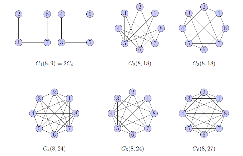
We have devised and implemented a backtracking algorithm to check if there is a distance magic graph for a given number of vertices \(n\) and a specific magic constant \(k\). Our algorithm is deterministic, and it explores all the possible solutions in a robust manner. We have implemented this algorithm to construct magic graphs for \(k = 28\) and \(32\). Our search for \(k = 16\) shows that no graph admits the magic constant \(16\). Additionally, with this algorithm, we have generated all distance magic graphs (up to isomorphism) of order up to \(12\) (see Table 1). This enhances the existing collection of distance magic graphs given in [16]. In particular, we find a new sixth graph of order \(8\), adding to the list of \(5\) such graphs given in [16].
This algorithm serves as a practical tool for researchers and enthusiasts in the field of distance magic graphs. Addressing the general challenge of characterizing all graphs possessing distance magic labelings using algorithms presents a computational hurdle. This is mainly due to the impracticality of generating all non-isomorphic graphs since this becomes increasingly unfeasible as the graph order grows. Consequently, the algorithms devised for characterization problems often encounter limitations or become computationally intensive when dealing with graphs of larger vertices.
It is believed that for a given \(n\), only a small subset of the set of all graphs of order \(n\) possesses the distance magic property. Consequently, a different approach is required rather than providing a collection of non-isomorphic graphs as input and subsequently characterizing them for the distance magic property. Instead, the focus shifts towards developing algorithms capable of dynamically constructing all distance magic graphs on \(n\) vertices. By adopting this strategy, we can bypass the challenge of generating all non-isomorphic graphs. We have successfully implemented this approach.
Let \(G\) be a graph. A subset \(S\) of the vertex set of \(G\) is said to be a dominating set if there is a function \(f:V \to \{0,1\}\), called dominating function, such that \(f(S) = \{1\}\), \(f(V \backslash S) = \{0\}\) and for each vertex \(v \in V \backslash S\), \(\sum_{u \in N(v)}f(u) \ge 1\). The domination number \(\gamma(G)\) of a graph is given by \[\gamma(G) = \min\{|f| : f \text{ is a dominating function}\},\] where \(|f| = \sum_{v \in V}f(v)\). There is another variation of domination called fractional domination.
This concept of a fractional domination number has a close relation with the magic constant of a graph as stated in the following theorem.
It is known that a \(2\)-regular graph \(G\) is distance magic if and only if it is a disjoint union of copies of cycle \(C_4\) [6]. Further, each positive integer of the form \(4t+1\) is a magic constant of a graph union of \(t\) copies of a \(4\)-cycle \(tC_4\) as stated in the following theorem.
The following result shows that each positive integer of the form \(4t+3\) is a magic constant of a graph \(P_3 \cup tC_4\).
\(k=n\).
\(\delta(G) = 1\).
Either \(G\) is isomorphic to \(P_3\) or \(G\) contains exactly one copy of \(P_3\) and all other components are isomorphic to \(C_4\).
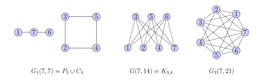
Figure 2 shows the distance magic
labeling of \(P_3 \cup 2C_4\) with
magic constant \(11\).
From Theorems 2.6 and 2.7, we conclude that all odd positive integers \(\ge 3\) are magic constants. This also answers the question: does \(p^{t}, t\ge 1\) belong to the set of magic constants, where \(p\) is odd prime? (see [7]).
Now, we explore the case of the even positive integers, which are
magic constants.
When \(H\) is an arbitrary graph with
vertices \(x_1,x_2 \dots, x_n\), and
\(G\) is any graph with \(t\) vertices, then by \(H[G]\) we denote the graph, which arises
from \(H\) by replacing each vertex
\(x_i\) by a copy of the graph \(G\) with vertex set \(X_i = \{x_{i_1}, \dots, x_{i_t}\}\), and
each edge \(x_ix_j\) by the edges of
the complete bipartite graph \(K_{t,t}\) with bipartition \(X_i,X_j\). The graph \(H[G]\) is then called lexicographic
product or the composition of \(H\) and \(G\).
In [9], the authors proved that for an \(r\)-regular graph \(G\) on \(n\) vertices, the magic constant of \(G[\overline{K_{2t}}]\) is \(k = rt(2nt + 1)\). With \(r = 2\) and \(t = 1\), we obtain \(k = 4n+2\). This gives the proof of the following theorem.
In [8], the authors proved that there exists a \(4\)-regular distance magic graph \(G=(V,E)\) of odd order if and only if \(|V| \ge 17\). Now, we use this result to prove the existence of even magic constants of the form \(4t+4\), \(t \ge 8\).
Proof. Let \(G\) be a \(4\)-regular distance magic graph of odd order. Then, \(|V(G)| \ge 17\). By Corollary 2.4, the magic constant \(k\) of this graph \(G\) is given by \(k = \frac{4(|V|+1)}{2} = 2|V|+2\). If we write \(|V| = 2t+1\), where \(t \ge 8\), then \(k = 4t+4\). This proves the theorem. ◻
Proof. We know that, if \(16\) is a magic constant of an \(r\)-regular graph \(G\) on \(n\) vertices then by Corollary 2.4, \(k = \frac{r(n+1)}{2}\) and \(n \le k\). This implies \(n = \frac{32}{r} – 1\). Since \(n\) is an integer, we have \(r = 1, 2, 4, 8, 16\), or \(32\). Since \(G\) is \(r\)-regular graph on \(n\) vertices, we must have \(n > r\). Therefore, we discard the possibilities \(r = 8, 16\) and \(32\). With \(r=4\) we get \(n=7 < 17\). Therefore, by Theorem 2.5, \(r=4\) is not possible, and hence we discard this possibility. There cannot be \(1\)-regular distance magic graph on \(32\) vertices. Therefore, we discard the case \(r = 1\). Recall that, if \(r= 2\) then \(G\) is union of disjoint copies of \(C_4\). Hence, by Theorem 2.6, the magic constant \(k \equiv 1 \pmod{4}\). But \(k = 16\) and \(16 \not \equiv 1 \pmod{4}\). Therefore, we discard the case \(r = 2\). This completes the proof. ◻
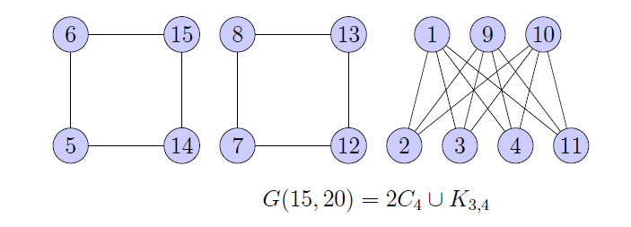
We already know that the integers \(1, 2, 4, 6, 8\) and \(12\) are not magic constants [7], while \(10\), \(20\) [7], and \(24\) [16] are magic constants, as shown in Figures 3, 6, 8, respectively. Also, we will see in Section 3 that these distance magic graphs can also be generated using our algorithm with the given magic constants. Theorems 2.9 and 2.10 provide further insights into the nature of the set of magic constants. Theorem 2.9 reveals that all positive integers congruent to \(2~(\bmod\ 4)\), with the exceptions of \(2\) and \(6\), are the members of the set of magic constants. Meanwhile, Theorem 2.10 establishes that all positive integers greater than or equal to \(36\) and congruent to \(0~(\bmod\ 4)\) are also in the set of magic constants.
As a result, the only remaining even positive integers requiring examination as magic constants are \(16\), \(28\), and \(32\). We devise an algorithmic approach to determine whether these integers qualify as magic constants of some graphs. Thus, we obtain a complete characterization of all magic constants (see Theorem 5.1).
Consider the following example given in [12]: If the generalized Myclielskian of the complete bipartite graph \(\mu_{m}(K_{a,b})\) is distance magic, then by Theorem 2.2, its magic constant is given by \(k = \frac{(m(a+b) + a+b+1)(m(a+b) + a+b+2)}{2m+3}\). When \(a=b=1\), then \(k = 2m+4\), which is an integer, but \(K_{1,1} \cong K_2\) and \(\mu_m(K_2)\) is not distance magic. On the other hand, for the case where \(a = b = 2\) and \(m \ge 1\), \(k\) is an integer \(8m + 10\) and \(\mu_{m}(K_{2,2})\) is distance magic. When \(k\) is not an integer, Theorem 2.2 implies that \(G\) is not distance magic. However, when \(k\) is an integer \(G\) may or may not be distance magic.
Therefore, it is noteworthy that given a graph \(G\) and the exact value of \(\gamma_{ft}(G)\), one can compute the value of (the magic constant) \(k\), but it is not possible to decide whether the underlying graph \(G\) is distance magic or not using Theorem 2.2. Even if the fraction \(\frac{n(n+1)}{2\gamma_{ft}(G)}\) is an integer, the graph \(G\) may or may not be distance magic.
The algorithm that we describe below is a natural way to construct distance magic graphs, and it has been adopted previously for smaller order graphs (see Chapter 2, [7]). Here, we give a general and robust version of the same.
Given positive integers \(n\) and \(k\), our algorithm checks if there exists a distance magic graph with vertex set \(\{1,2, \dots, n\}\) and a magic constant \(k\). We denote such graphs as \(G(n,k)\). Without loss of generality, we may assume that each vertex \(i\) is labeled as \(i\) for \(1 \le i \le n\). The algorithm returns the first successful search if such a distance magic graph exists.
Let \(S\) be the set of all subsets of the set \(\{1,2, \dots, n\}\) with the sum of its elements equal to \(k\). For each \(1 \le i \le n\), let \(NS(i) = \{T \in S: i \not \in T\}\). Note that if there exists a distance magic graph \(G(n,k)\), then the neighborhood of a vertex \(i\), \(N(i)\), is a member of \(NS(i)\). Next, fix a neighborhood of a vertex \(n\), that is, an element of \(NS(n)\), and construct a tree rooted at \(N(n)\) in the following manner. At level \(0\), we have only the root node. Add all elements in \(NS(n-1)\) as children to \(N(n)\). This is level \(1\). Add elements of \(NS(n-2)\) as children to each node in level \(1\). This is level \(2\). Continue until we add all elements in \(NS(1)\) to each node in level \(n-1\). Note that at level \(i \ge 1\), each node of this tree \(T(n,k)\) is a possible candidate for a \(N(n-i)\). Each branch of this tree \(T(n,k)\) gives an adjacency list for the vertices \(1,2, \dots, n\). These lists may or may not correspond to a graph. Whenever adjacency lists corresponding to a branch give a graph, we call such a branch a successful branch.
The algorithm consists of the following steps:
Generate all subsets of the set \(\{1,2, \dots, n\}\) that have the sum of its elements equal to \(k\).
For each vertex \(1 \le i \le n\), construct \(NS(i)\).
Construct a rooted tree \(T(n,k)\) with a root as a fixed element of \(NS(n)\).
For a tree \(T(n,k)\) obtained in Step (\(3\)), find a successful branch. Repeat Steps (\(3\)) and (\(4\)) for each element of \(NS(n)\) until we find a successful branch or run out of elements in \(NS(n)\).
To optimize the search space, we merge Step \((3)\) and Step \((4)\) into a new streamlined Step (\(3'\)), as below.
We explore the branches of \(T(n,k)\) as discussed in Step \((3)\) and Step \((4)\) with the following condition. Let the tree be constructed to the level \(i (0 \le i \le n-2)\) and \(NS(n-i) = \{s_1, s_2, \dots, s_{t_i}\}\), \(NS(n-(i+1)) = \{r_1, r_2, \dots, r_{t_{h}}\}\). Next, while adding children \(r_b\) at level \(i+1\) to any of the nodes \(s_a\) we will check the following two conditions. \[\label{eq: check1} n-(i+1) \text{ is in any of it's ancestors at level } j \le i \text{ if and only if } n-j \in r_b . \tag{1}\]
and \[\label{eq: check2} \text{neighborhood sum of } s_a \text{ does not exceed } k. \tag{2}\]
The part \((1)\) of the Step (\(3'\)) ensures symmetry, which means that \(u\) is adjacent to \(v\) if and only if \(v\) is adjacent to \(u\). The part \((2)\) of Step (\(3'\)) ensures that the neighborhood sum of any vertex at any stage does not exceed the magic constant \(k\). Although this condition may not seem critical at this point, it plays a crucial role in controlling the growth of the tree (see Section 3.3). If at least one of the conditions (1) or (2) stated in Step \(3'\) are not met at any step, we avoid adding the corresponding node, preventing further growth of the tree below that node. This reduction strategy significantly reduces the order and therefore the size of the tree \(T(n,k)\), leading to an exponential reduction in the search space.
Step (\(1\)) uses backtracking to generate subsets of \(\{1, 2, \dots, n\}\) of the given sum \(k\). The Step (\(3'\)) of the algorithm involves a backtracking strategy in the process of finding a successful branch in the constructed tree \(T(n,k)\). The algorithm systematically explores the branches of each rooted tree, corresponding to a different choice of elements from the set \(NS(n)\). If, during this exploration, it is determined that a particular branch cannot lead to success, the algorithm backtracks to the previous decision point and explores alternative branches. This backtracking mechanism allows for an exhaustive search of the solution space, ensuring that all possible combinations of elements are considered. The backtracking in Step (\(3'\)) is crucial to efficiently navigate the complex solution space represented by the tree, avoiding unnecessary computations and ultimately identifying successful branches of \(T(n,k)\).
We provide the pseudocode for the algorithm in the Appendix.
It is sufficient to prove that every \(G(n,k)\) graph corresponds to a (successful) branch of some \(T(n,k)\) and each successful branch of each \(T(n,k)\) corresponds to some graph \(G(n,k)\). This follows by observing that if \(T(n,k)\) has a successful branch, then the nodes on that branch constitute a graph \(G(n,k)\).
Conversely, suppose that there is a graph \(G(n,k)\). Consider a tree \(T(n,k)\) rooted at some element \(r\) of \(NS(n)\). There is a one-to-one correspondence between branches of \(T(n,k)\) and the elements of the cartesian product \(NS(n-1) \times NS(n-2) \times \dots \times NS(1)\). The neighborhood \(N(i)\) of each vertex \(i\) is a member of \(NS(i)\). Hence, \((N(n-1), N(n-2), \dots, N(1))\) is an element of the cartesian product \(NS(n-1) \times NS(n-2) \times \dots \times NS(1)\). Thus, it corresponds to some branch of \(T(n,k)\). This establishes the correctness of the algorithm.
Let us illustrate the steps of our algorithm with \(G(7,7)\). By Theorem 2.7, we know that there is only one graph \(P_3 \cup C_4\) up to isomorphism on \(7\) vertices admitting the magic constant \(7\). All subsets of the set \(\{1,2, \dots, 7\}\) having sum \(7\) are: \[\nonumber \bigr[[7],\; [6, 1],\; [5, 2],\; [4, 3],\; [4, 2, 1] \bigr].\]
We have listed all the subsets as a list of lists for the proper indexing purpose in the pseudocode. This completes Step \(1\). Next, we generate all possible neighborhood sets for each vertex as suggested in Step \(2\). \[\begin{aligned} \nonumber &NS(1) = \bigr[[7],\; [5, 2],\; [4, 3] \bigr]\\ &NS(2) = \bigr[[7],\; [6, 1]\; [4, 3] \bigr]\\ &NS(3) = \bigr[[7],\; [6, 1],\; [5, 2],\; [4,2,1] \bigr]\\ &NS(4) = \bigr[[7],\; [6,1],\; [5, 2] \bigr]\\ &NS(5) = \bigr[[7], \; [6,1],\; [4, 3]\; [4, 2, 1] \bigr]\\ &NS(6) = \bigr[[7],\; [5, 2],\; [4, 3],\; [4, 2, 1] \bigr]\\ &NS(7) = \bigr[[6, 1],\; [5, 2],\; [4, 3],\; [4, 2, 1] \bigr] \end{aligned}\]
Now we construct a tree \(T(7,7)\) rooted at the node \([6,1]\) from \(NS(7)\). This makes \(N(7) = [6, 1]\). Add all elements of the set \(NS(6)\) as children to the root node as shown in Figure 4. The set of possible candidates for \(N(6)\) is \[\nonumber NS(6) = \bigr[[7],\; [5, 2],\; [4, 3],\; [4, 2, 1] \bigr].\]
We have chosen \(NS(7) = [6, 1]\), to maintain symmetry as stated in (1) of Step \(3'\), we must have \(7 \in N(6)\). The only such element in \(NS(6)\) is \([7]\). Hence, we discard all other nodes in the level \(1\), and the tree won’t grow further below those nodes. Now we go to level \(2\). The set of possible candidates for \(N(5)\) is \[\nonumber NS(5) = \bigr[[7], \; [6,1],\; [4, 3]\; [4, 2, 1] \bigr].\] So far we have \(N(7) = [6, 1]\) and \(N(6) = [7]\). Since \(5 \not \in N(6) \cup N(7)\), \(6, 7 \not \in N(5)\) maintaining the condition given in (1) of Step \(3'\). Then the only choices for \(N(5)\) are \([4, 3]\) and \([4, 2, 1]\). Without loss of generality, consider \(N(5) = [4,3]\). Now we go to the level \(3\). The set of possible candidates for \(N(4)\) is \[\nonumber NS(4) = \bigr[[7],\; [6,1],\; [5, 2] \bigr].\]
So far we have \(N(7) = [6, 1]\), \(N(6) = [7]\) and \(N(5) = [4, 3]\). Here \(4 \not \in N(6) \cup N(7)\) hence \(6, 7 \not \in N(4)\) but \(4 \in N(5)\) hence \(N(4)\) must contain \(5\). The only choice for \(N(4)\) is \([5,2]\). We continue in a similar way, and lastly, we add pendants \([7]\), \([5,2]\), and \([4,3]\) from the set \(NS(1)\). For \(N(1)\) we discard the nodes \([5, 2]\) and \([4, 3]\) because \(1 \not \in N(j)\) for any \(j = 2, 3, 4, 5\) and \(N(1)\) must contain \(7\) since \(1 \in N(7)\), hence maintaining symmetry condition as given in (1) of Step \(3'\).
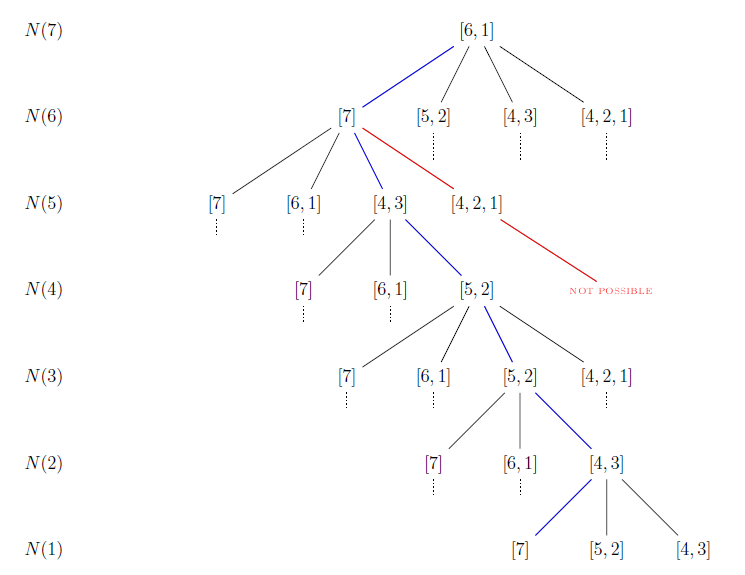
In Figure 4, we have illustrated a case of a successful branch (colored blue).
Now let us consider a case where we select the node \([4, 2, 1]\) instead of \([4, 3]\) at the level \(2\) (see the red colored branch in Figure 4). In this case, so far we have \(N(7)= [6, 1]\), \(N(6) = [7]\) and \(N(5) = [4, 2, 1]\). Then we go to level \(3\). The set of possible candidates for \(N(4)\) is: \[\nonumber NS(4) = \bigr[[7],\; [6,1],\; [5, 2] \bigr].\]
Since \(4 \not \in N(6) \cup N(7)\) but \(4 \in N(5)\), we must have \(6,7 \not \in N(4)\) but \(5 \in N(4)\). The only such possibility is \([5, 2]\). But then \(4,5 \in N(2)\) and the neighborhood sum of the vertex \(2\) is more than \(k = 7\). This violates the condition \((2)\) of Step \(3'\). Therefore, \(N(4)\) has no choices and we discard this unsuccessful branch. This discarded branch is shown in red color in Figure 4.
For a distance magic graph \(G\) on \(n\) vertices with distance magic labeling \(f\) and magic constant \(k\), it is easily seen that \(\sum_{v \in V}deg(v)f(v) = nk\) [14]. For any vertex \(v\), \(1 \le \delta(G) \le deg(v) \le \Delta(G) \le n-1\). Hence, we have an upper bound \(k \le \frac{n^2-1}{2}\). By the definition of the distance magic graph, \(k\) cannot be less than \(n\). Hence, we have \(n \le k \le \frac{n^2 -1 }{2}\), and the lower bound is sharp. Therefore, to check whether a given positive integer \(k\) is a magic constant, we need to run the algorithm for each pair \((n, k)\), where \(1 \le n \le k\). Let \(\alpha\) be the largest positive integer such that \(\frac{\alpha(\alpha+1)}{2} \le k\). Hence, running the algorithm for the pairs \((n, k)\), where \(\alpha \le n \le k\) is sufficient. For example, for \(k = 16\), the possibilities for \(n\) are \(6, 7, \dots, 16\). Further, we can omit a few values in some cases, as mentioned in (Chapter 2, [7]).
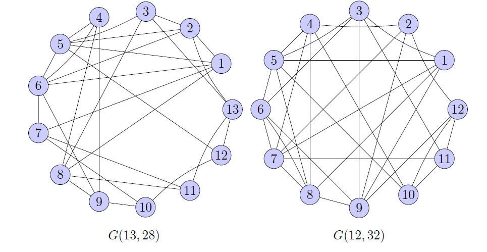
Our algorithm explores the possibility of \(k = 16\) being the magic constant for the graphs on a possible number of vertices \(n\). However, findings show that no graph admits the magic constant \(16\). The algorithm generates multiple graphs that admit \(28\) and \(32\) as magic constants. As a representative example, we list one of the such graphs in Figure 5. Due to the large number of non-isomorphic distance magic graphs of order \(11\) and \(12\) (see Table 1), we will list all non-isomorphic distance magic graphs of order up to \(10\) (see Section 4).
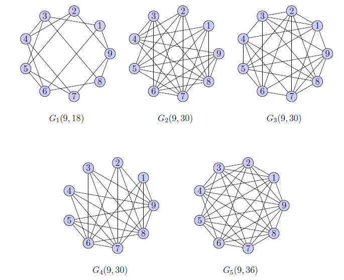
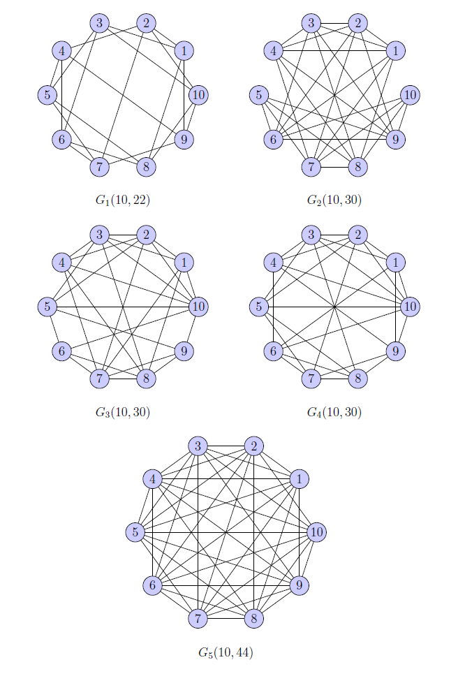
| number of vertices: \(n\) | \(3\) | \(4\) | \(5\) | \(6\) | \(7\) | \(8\) | \(9\) | \(10\) | \(11\) | \(12\) |
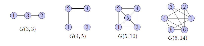
| number of non-isomorphic distance magic graphs | \(1\) | \(1\) | \(1\) | \(1\) | \(3\) | \(6\) | \(5\) | \(5\) | \(74\) | \(1160\) |
In this section, we list all non-isomorphic distance magic graphs of order up to \(10\) in Figures 6–10.
There is no known polynomial-time algorithm to generate distance magic graphs on a given number of vertices and a given magic constant. Our algorithm presented in Section 3 is practically implementable for considerably large order distance magic graphs. This algorithm can be extended to generate \(D\)-distance magic graphs introduced by O’Neal et al. [10]. Let \(G\) be a graph and let \(\sf{diam}(G)\) denote the diameter of \(G\). Let \(D \subset \{1,2, \dots, \sf{diam}(G)\}\) and let \(W\) be a multiset of positive real numbers of size equal to the number of vertices in \(G\). A graph \(G\) is said to be \(D\)-distance magic if there is a bijection \(f: V(G) \rightarrow W\) such that \(w(x) = k\) for all vertices \(x\), where \(w(x) = \sum_{\{y:d(y,x) \in D\}}f(y)\) and \(d(x,y)\) denotes the distance between \(x\) and \(y\).
With the results known earlier and those verified in this paper, the magic constants are now completely characterized, and we have the following theorem.
Not all magic constants arise from connected graphs. Also, for some integers, for example, \(n = k = 7\), there is a unique distance magic graph \(G(n,k)\). This naturally leads to the following questions.
Which magic constants are realized by connected distance magic graphs?
For which pairs \((n, k)\), there is unique distance magic graph on \(n\) vertices with magic constant \(k\)?
We conclude by observing that it would be interesting to find a non-algorithmic proof for the case \(k = 16\).
The authors are grateful to Atharva Karandikar and Satyaprasad for their invaluable assistance in implementing the algorithm.