
Consider an undirected graph \(G(V,E)\), where \(V\) represents the set of vertices and \(E\) denotes the set of edges [5]. The concept of graph energy, first introduced by Ivan Gutman [10,23] in 1978, emerged as a refined extension of the Hückel Molecular Orbital (HMO) theory, originally formulated to quantify the total \(\pi\)-electron energy in molecular systems.
Following this, the concept of graph energy resurfaced as a significant and highly researched theme within chemical graph theory [23], leading to a surge in academic attention, with more than a hundred research papers published annually [11,12]. Numerous properties and well-established bounds associated with graph energy have since been developed and explored extensively [2,3,6].A molecular graph \(G\) with \(n\) vertices. The eigenvalues of the \((0, 1)\)-adjacency matrix of \(G\), denoted by \(\lambda_1, \lambda_2, \dots, \lambda_n\), constitute the spectrum of \(G\). The total sum of the absolute values of the eigenvalues of \(A(G)\) defines the energy of the graph \(G\) [10,24].
In this framework, Patekar et al. introduced a novel concept called the pathway matrix [17,20], which leads to the definition of path energy for a graph, extending the classical notion of graph energy. Define a matrix \(P = (p_{ij})\) of dimension \(n \times n\), where for \(i \neq j\), \(p_{ij}\) represents the greatest number of vertex-disjoint paths from vertex \(v_i\) to vertex \(v_j\). For the case where \(i = j\), set \(p_{ij} = 0\). In the paper by Sabeen et al. [19], the author explores the \(P^{(k)}\) pathway energy across various graph classes, deriving key conclusions about the behavior of \(P^{(k)}\) path energy. Similarly, Raza et al. [18] in 2023 dig into the spectrum of graphs. In a related study, Xu and Zhou [22] identify the graphs that attain both upper and lower bounds on the path index for graphs with specified structural parameters. In the book by Cvetkovski et al. [7], the authors examine a variety of inequalities, some of which serves as key instruments in tightening the bounds and enhancing the precision of energy calculations within graph structures. We utilize these tools to derive improved upper and lower bounds on the pathway energy for graphs with suitable parameters. Hutter et al. [13] explored the use of machine learning to predict algorithm runtime based on problem-specific features. A simulation of graphs for reduced order modelling in city-scale district energy grids, leveraging spectral graph theory, was recently proposed by Simonsson et al. [21]. Duraj and Mezic [9,15] introduced a novel complexity measure for directed graphs, termed spectral complexity. The spectrum of the path matrix, can be optimally resolved in polynomial time, despite the inherent complexity of the graphs.
Graph theory is fundamental in optimizing complex networks, yet calculating pathway energy, key to measuring network connectivity through vertex-disjoint paths-poses significant challenges. Efficient computation of pathway energy is critical for designing robust and high-performing networks. To address the complexity of calculating pathway energy for intricate flower families, we propose a novel algorithmic approach.
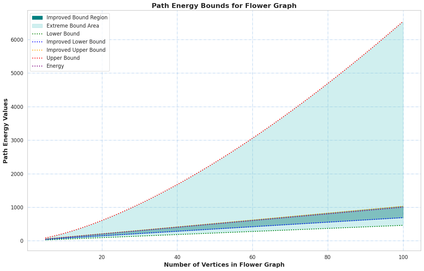
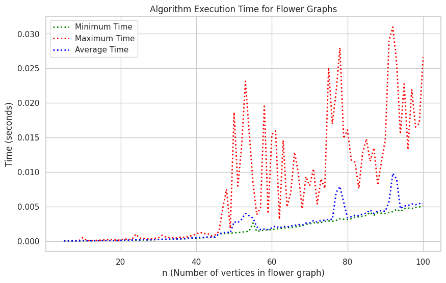
Our method constructs a matrix \(P\) that represents the maximum number of non-overlapping paths between distinct vertex pairs. From the characteristic values of \(P\), we derive pathway energy bounds, including upper, lower, improved upper, improved lower, and exact limits. We further develop an algorithm that performs \(n\)-trial analyses to assess the time complexity of these graphs, by determining average, maximum, and minimum execution times. This approach not only reveals computational challenges across various graph configurations but also provides a streamlined algorithmic framework. By combining advanced mathematical techniques with innovative algorithms, our study offers new insights into network complexity, significantly enhancing both theoretical understanding and practical applications in graph theory.
In this section, the ideas and inequalities that provide the foundation for our work were discussed.
\[\label{1} \left(\sum\limits_{i=1}^{n} a_i b_i\right)^2 \leq \left(\sum\limits_{i=1}^{n} a_i^2\right) \left(\sum\limits_{i=1}^{n} b_i^2\right). \tag{1}\]
The different pathway energy extremities such as lower, upper, improved upper, and improved lower bounds for the flower graph families are explored in this section.
\(\sum\limits_{i=1}^{2n+1} \mu_i^2 = 4\Lambda +3\curlyvee +2\top.\)
Proof. Let us examine the vertex-disjoint pathway matrix
\(A_p(F_n)\) associated with a flower
graph. The elements of this matrix can be expressed in a structured
manner:
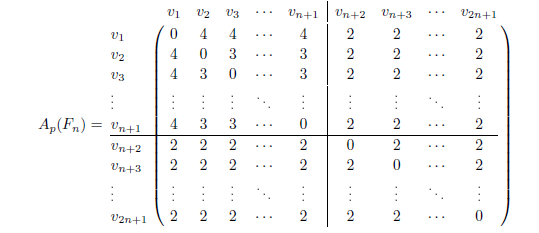
The lower bound of pathway energy is given by: \[E_p(F_n) \geq \sqrt{4\Lambda+ 3\curlyvee + 2\top + \frac{2}{(l)(l-1)}\prod_{i=1}^{l} (\mu_i^{w_i})^2},\] where \(w_i\) are the weights, \(\sum_{i=1}^{l} w_i = 1\) gives the total sum of the characteristic value weights.
The improved lower bound of pathway energy is: \[E_p(F_n) \geq \sqrt{4\Lambda+ 3\curlyvee + 2\top + (l)(l-1) D^ {\frac{2}{l}}}\quad \text{where}\, \quad D = |\det A_p(F_n)|.\]
Proof. Consider the flower graph \(F_n\) with an vertex-disjoint pathway matrix of order \(l \times l\), where \(l = 2n+1\) represents the vertices. The characteristic values \(\mu_1, \mu_2, \dots, \mu_l\) are obtained by solving the characteristic polynomial \(|A_p(F_n) – \mu I| = 0\). The pathway energy \(E_p(F_n)\) is the sum of the absolute values of the characteristic values of the vertex-disjoint path matrix. The following condition describes this. \[^2 = \left(\sum\limits_{i=1}^{l}|\mu_i|\right)^2 .\]
Moreover, this can also be written as the product of the absolute characteristic value summations:
\([E_p(F_n)]^2 = \left(\sum\limits_{i=1}^{l}|\mu_i|\right)\left(\sum\limits_{j=1}^{l}|\mu_j|\right)\).
\([E_p(F_n)]^2 = \left(\sum\limits_{i=1}^{l}|\mu_i|^2\right) + \left(\sum\limits_{i\neq j}|\mu_i| |\mu_j|\right).\)
Case 1: Proof for the pathway energy lower bounds of flower graph
From the Chebyshev’s Inequality 3, we derive that, \[^2 \geq {\sum_{i=1}^{l}|\mu_i|^2 + \frac{2}{l(l-1)} \left( \sum_{i=1}^{l} |\mu_i| \right) \left( \sum_{i=1}^{l} |\mu_i| \right)}.\]
From the Weighted AM–GM inequality 4, we conclude, \[\begin{aligned} \left[E_p\left(F_n\right)\right]^2 &\geq{\sum_{i=1}^{l}|\mu_i|^2 + \frac{2}{l(l-1)} \left( \sum_{i=1}^{l} \mu_i w_i \right) \left( \sum_{i=1}^{l} \mu_i w_i \right)}\quad \text{where} \sum_{i=1}^{l} w_i = 1, \\ &\geq {\sum_{i=1}^{l}|\mu_i|^2 + \frac{2}{l(l-1)} \prod_{i=1}^{l} \left(\mu_i^{w_i} \right) \prod_{i=1}^{l} \left(\mu_i^{w_i} \right)}, \\ &\geq {4\Lambda+ 3\curlyvee + 2\top + \frac{2}{l(l-1)} \prod_{i=1}^{l} \left(\mu_i^{w_i} \right)^2}.\text {…………. [by Theorem 4.1]}. \end{aligned}\]
Thus, the lower bounds of the pathway energy for flower graph is, \[E_p(F_n)\geq \sqrt{4\Lambda+ 3\curlyvee + 2\top+\frac{2}{l(l-1)} \prod_{i=1}^{l} \left(\mu_i^{w_i} \right)^2}.\]
Case 2: Proof for the pathway energy improved lower bounds.
From the AM-GM inequalities in Eq. (2), we derive that \[\frac{1}{l(l-1)} \sum_{\substack{ i \neq j}} |\mu_i||\mu_j| \geqslant \left( \prod_{\substack{i \neq j}} |\mu_i||\mu_j| \right)^{\frac{1}{l(l-1)}},\]
\[\begin{aligned} {\left[E_p\left(F_n\right)\right]^2} &\geq \sum_{i=1}^{l} \left|\mu_i \right|^2+l(l-1) \left(\prod_{i \neq j}\left|\mu_i \right|\left|\mu_j\right|\right)^{\frac{1}{l(l-1)}}\\ & =\sum_{i=1}^{l}\left|\mu_i\right|^2+l(l-1) \left|\prod_{i=1}^{l} \left(\mu_i\right)\right|^{\frac{2}{l}} \\ & ={4\Lambda+ 3\curlyvee + 2\top+l(l-1) D^{\frac{2}{l}}} \quad { \text {by Theorem 4.1}}. \end{aligned}\]
Thus, the improved lower bounds of the pathway energy for flower graph is, \[E_p(F_n)\geq \sqrt{4\Lambda+ 3\curlyvee + 2\top+l(l-1) D^{\frac{2}{l}}}.\] ◻
The upper bound of pathway energy is given by: \(E_p(F_n)\leq \sqrt{l(4\Lambda+ 3\curlyvee + 2\top)}\)
The improved upper bound of pathway energy is: \(E_p(F_n)\leq \sqrt{5(4\Lambda+ 3\curlyvee + 2\top)}.\)
Proof. The methodology employed to ascertain the characteristic values echoes that utilized in Theorem 4.2. Let \(\mu_1 \geq \mu_2 \geq \mu_3 \geq \dots \geq \mu_{n-1} \geq \mu_{n} \geq \dots \geq \mu_{l}\) denote the characteristic values of the \(l \times l\) vertex-disjoint path matrix of \(F_n\).
Case 1: Proof for the pathway energy upper bound of flower graph.
From the Cauchy-Schwarz inequality in the Eq. (1) we derive that, \[\left(\sum\limits_{i=1}^{l} \alpha_i \beta_i\right)^2 \leq \left(\sum\limits_{i=1}^{l} \alpha_i^2\right) \left(\sum\limits_{i=1}^{l} \beta_i^2\right).\]
To establish the upper bound, consider the expression \([E_p(F_n)]^2 \leq \left(\sum_{i=1}^{l} \alpha_i \beta_i\right)^2\), where the pathway energy is bounded by the right-hand side. Substituting \(\alpha_i = 1\) and \(\beta_i = |\mu_i|\) into the inequality yields the desired result.
\[\begin{aligned} ^2 & \leq \left( \sum\limits_{i=1}^{l} 1.|\mu_i|\right)^2 \leq \left( \sum\limits_{i=1}^{l} 1 \right)^2 .\left( \sum\limits_{i=1}^{l} |\mu_i|^2\right) \text {……………… by 1)},\\ &= l(4\Lambda+ 3\curlyvee + 2\top) \text {…………………. by Theorem 4.1},\\ [E_p(F_n)] & \leq \sqrt{l(4\Lambda+ 3\curlyvee + 2\top)}. \end{aligned}\]
Thus, the upper bound of the pathway energy of the flower graph concluded by, \[E_p(F_n)\leq \sqrt{l(4\Lambda+ 3\curlyvee + 2\top)}.\]
Case 2: Proof for the pathway energy improved upper bound.
The Weighted Cauchy Schwarz inequality in (5) allows us to deduce that,
\[\left(\sum\limits_{i=1}^{l} a_ib_iw_i\right) ^2 \leq \left (\sum\limits_{i=1}^{l} a_i^2w_i\right) \left(\sum\limits_{i=1}^{l} b_i^2w_i\right).\]
For proving the improved upper bound, consider \([E_p(F_n)]^2 \leq \left( \sum\limits_{i=1}^{l}a_{i}.b_{i}.w_i\right)^2\), such that the pathway energy of the graph is less than RHS of the inequality, and substituting \(a_{i}=\frac{1}{(l)^{\frac{3}{2}}}\,|\mu_i|\) and \(b_{i}=1\) \(w_i=\sqrt{5}\), in the above inequality,
\[\begin{aligned} ^2 & \leq \left( \sum\limits_{i=1}^{l} \frac{\mu_i^2}{(l)^3}.\sqrt{5}\right) \left( \sum\limits_{i=1}^{l} 1.\sqrt{5}\right),\\ &\leq \frac{\sqrt{5}l}{l^3}\left( \sum\limits_{i=1}^{l} \mu_i^2 \right) .l^2\sqrt{5},\\ &= 5(4\Lambda+ 3\curlyvee + 2\top) \text {……………………. by Theorem 4.1},\\ [E_p(F_n)] & \leq \sqrt{5(4\Lambda+ 3\curlyvee + 2\top)}. \end{aligned}\]
Thus, the improved upper bound of the pathway energy for flower graph is, \[[E_p(F_n)] \leq \sqrt{5(4\Lambda+ 3\curlyvee + 2\top)}.\] ◻

The different pathway energy bounds of sunflower graph \(SF_n\) like lower, upper, improved lower, and improved upper bounds are investigated in this section.
Proof. The structure of the vertex-disjoint path matrix
\(A_p(SF_n)\) for the sunflower graph
is depicted as follows, 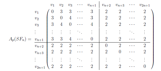
In this instance, \(\delta,\varkappa, \text{ and } \varphi\) denote the total of all elements 4, 3, and 2 respectively, present in the vertex-disjoint path matrices. ◻
The lower bound of pathway energy is given by: \[\begin{aligned} E_p(SF_n) \geq \sqrt{4\delta+3 \varkappa + 2 \varpi + \frac{2}{l(l-1)}\prod_{i=1}^{l} (\mu_i^{w_i})^2}, \end{aligned}\] where \(w_i\) are the weights, \(\sum_{i=1}^{l} w_i = 1\) gives the total sum of the characteristic value weights.
The improved lower bound of pathway energy is: \[\begin{aligned} E_p(SF_n) \geq \sqrt{4\delta+3 \varkappa + 2 \varpi + (l)(l-1) D^ {\frac{2}{l}}}\quad \text{where}\quad D = |\det A_p(SF_n)|. \end{aligned}\]
Proof. The proof is similar to Theorem 4.2 and is left to the interest of the reader. ◻
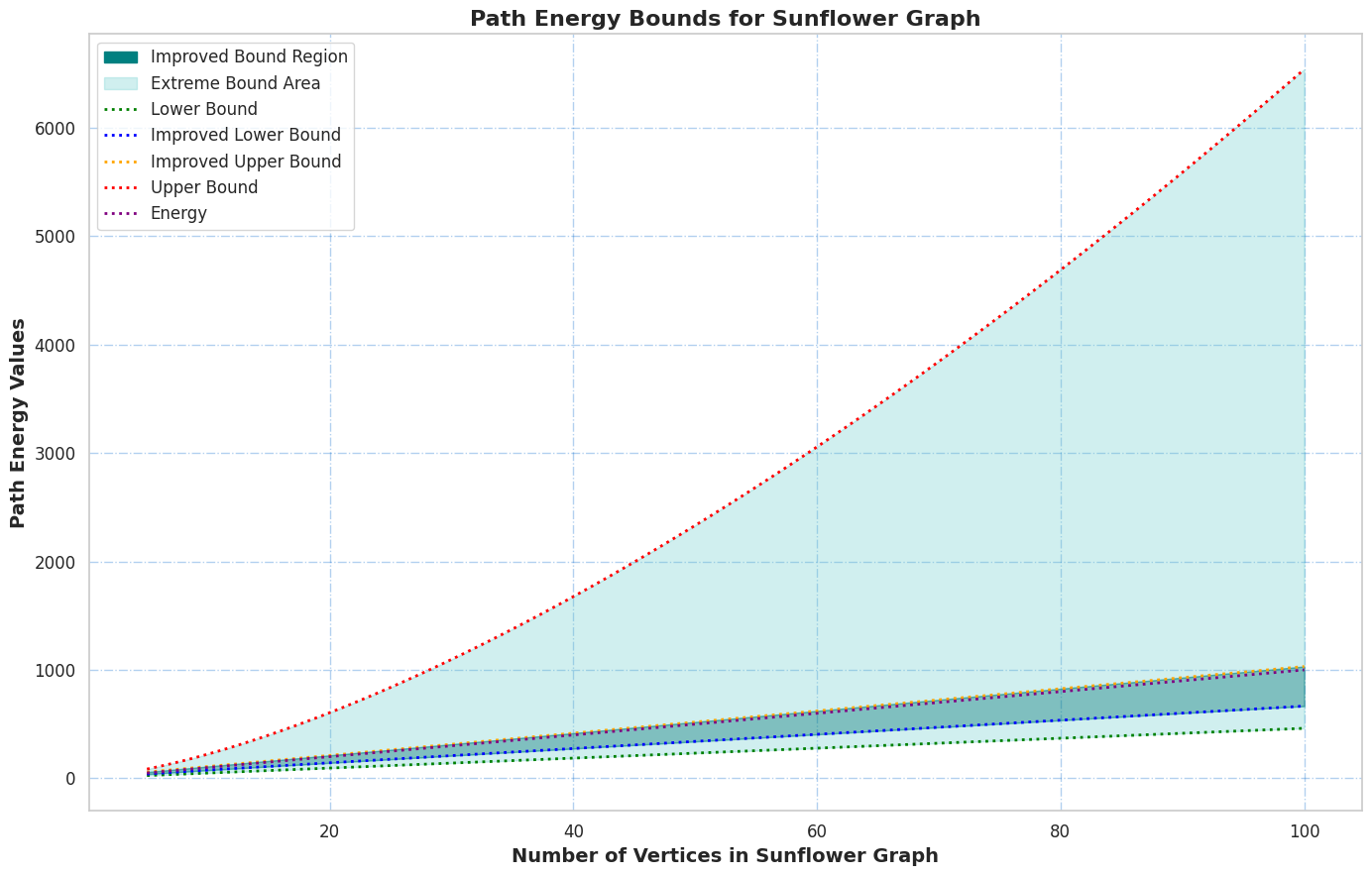
The upper bound of pathway energy is given by: \(E_p(SF_n)\leq \sqrt{l(4\delta+3\varkappa+2\varpi)}\)
The improved upper bound of pathway energy is: \(E_p(SF_n)\leq \sqrt{5(4\delta+3\varkappa+2\varpi)}.\)
Proof. The proof is similar to Theorem 4.4 and is left to the interest of the reader. ◻

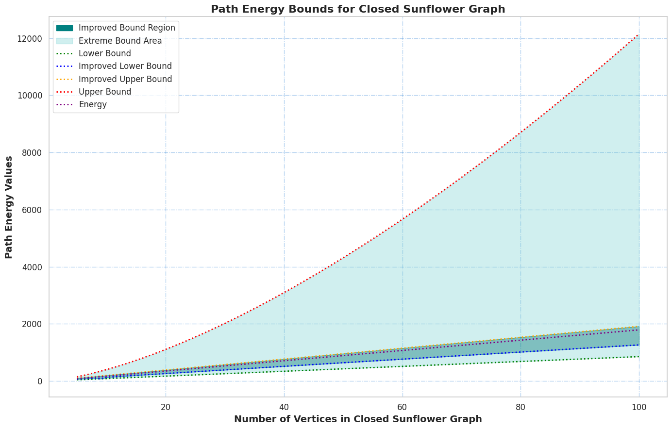
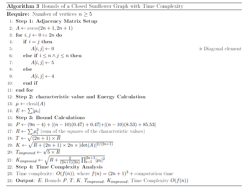
This section explicates the distinct path energy bounds for the closed sunflower graph \(CSF_n\), comprising the lower, upper, exact energy, improved lower and upper bound.
Proof. The arrangement of elements in the vertex-disjoint
path matrix \(A_p(CSF_n)\) of a closed
sunflower graph is shown below: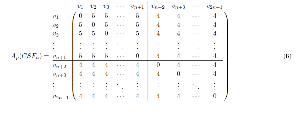
The characteristic equation associated with this \(2n+1 \times 2n+1\) square matrix is: \[a_{0}\mu^{2n+1} + a_{1}\mu^{2n} + a_{2}\mu^{2n-1}
+ \ldots + a_{n} = 0,\] where the characteristic values are
denoted as \(\mu_1, \mu_2,
\dots,\mu_{n-1},\mu_n,\dots, \mu_{2n+1}\).
The squared sum of these characteristic values is expressed as, \[\begin{aligned}
\sum_{i=1}^{2n+1} \mu_i^2= &
{\left[\sum_{i=j}^{2n+1}\left(\lambda_{i
j}\right)\right]+\left[\sum_{i<j}^{n+1}\left(\kappa_{i
j}\right)+\sum_{i>j}^{n+1}\left(\kappa_{i j}\right) \right]} \\
& +\left[\left(\sum_{i=1}^n \sum_{j>n}^{2n+1}\left(\chi_{i
j}\right)\right)+\left(\sum_{i>n}^{2n+1} \sum_{j=1}^{2
n+1}\left(\chi_{i j}\right)\right)+\left(\sum_{i>n+1}^{2n+1}
\sum_{j>n+1}^{2n+1}\left(\chi_{i j}\right)\right)\right] \\
= &\ 0\left(\alpha\right)+5\left(\kappa\right)+ 4\left(\chi\right)\\
= &\ 5\kappa + 4\chi.
\end{aligned}\]In this context, \(\kappa \text{ and } \chi\) represent the
sums of all the elements 5 and 4 in the path matrices,
respectively. ◻
The lower bound of pathway energy is given by, \[E_p(CSF_n) \geq \sqrt{\ 5\kappa + 4\chi + \frac{2}{l(l-1)}\prod_{i=1}^{l} (\mu_i^{w_i})^2},\] where \(w_i\) is the weights of the characteristic values and their sum is \(\sum_{i=1}^{l} w_i = 1\).
The improved pathway energy lower bound is given by, \[E_p(CSF_n) \geq \sqrt{\ 5\kappa + 4\chi+ l(l-1) D^ {\frac{2}{l}}} \quad \text{where } D = |\det A_p(CSF_n)|.\]
Proof. The vertex-disjoint path matrix of the closed sunflower network \(CSF_n\) has order \(l \times l\), where the vertices are represented by \(l = 2n+1\). Solving the polynomial equation \(|A_p(CSF_n) – \mu I| = 0\) yields the characteristic values \(\mu_1, \mu_2, \ldots, \mu_l\). Following the method in Theorem 4.2 and using terminology that has already been explained, the pathway energy \(E_p(CSF_n)\) is defined as the total of the absolute values of these characteristic values.
\([E_p(CSF_n)]^2 = \left(\sum\limits_{i=1}^{l}|\mu_i|\right)^2 + \left(\sum\limits_{i\neq j}|\mu_i| |\mu_j|\right)\).
Case 1: Proof for the pathway energy lower bound of \(\bf{CSF_n}\)
From the Chebyshev’s Inequality (3), we derive that, \[^2 \geq {\sum_{i=1}^{l}|\mu_i|^2 + \frac{2}{l(l-1)} \left( \sum_{i=1}^{l} |\mu_i| \right) \left( \sum_{i=1}^{l} |\mu_i| \right)}.\]
From the Weighted AM–GM inequality (4), we conclude, \[\begin{aligned} {\left[E_p\left(CSF_n\right)\right]^2} &\geq{\sum_{i=1}^{l}|\mu_i|^2 + \frac{2}{l(l-1)} \left( \sum_{i=1}^{l} \mu_i w_i \right) \left( \sum_{i=1}^{l} \mu_i w_i \right)}\quad \text{where}\;\;\; \sum_{i=1}^{l} w_i = 1, \\ &\geq {\sum_{i=1}^{l}|\mu_i|^2 + \frac{2}{l(l-1)} \prod_{i=1}^{l} \left(\mu_i^{w_i} \right) \prod_{i=1}^{l} \left(\mu_i^{w_i} \right)} \\ &\geq {\ 5\kappa + 4\chi+ \frac{2}{l(l-1)} \prod_{i=1}^{l} \left(\mu_i^{w_i} \right)^2}\text {……………. by (Theorem 6.1)}. \end{aligned}\]
Thus, the lower bound is \[E_p(CSF_n)\geq \sqrt{\ 5\kappa + 4\chi+\frac{2}{l(l-1)} \prod_{i=1}^{l} \left(\mu_i^{w_i} \right)^2}.\]
Case 2: Proof for the pathway energy improved lower bound.
From the AM-GM inequalities in Eq. (2), we derive that
\[\begin{aligned} {\left[E_p\left(CSF_n\right)\right]^2} & =\sum_{i=1}^{l}\left|\mu_i\right|^2+l(l-1) \left|\prod_{i=1}^{l} \left(\mu_i\right)\right|^{\frac{2}{l}} ={\ 5\kappa + 4\chi+l(l-1) D^{\frac{2}{l}}} \quad { \text {[by Theorem 6.1]}}. \end{aligned}\]
Thus, the improved lower bound of the pathway energy for closed sunflower graph is, \[E_p(CSF_n)\geq \sqrt{5\kappa + 4\chi+l(l-1) D^{\frac{2}{l}}}.\] ◻
Proof. The vertex-disjoint path configuration of the \(CSF_n\) graph is elaborated in detail in the path adjacency matrix (6). It has \(2n+1\) roots, implying that it contains \(2n+1\) characteristic values.
The characteristic equation of (6) is \[\label{18} (-\mu)^{2n+1} + \operatorname{tr}(-\mu)^{2n} + \cdots + \det (A_{p}(CSF_{n})) = 0. \tag{7}\]
Upon solving the Eq. (7), the \(2n+1\) characteristic values are determined to be,
\[\mu_1 = \mu_2 = \mu_3 = \cdots = \mu_{n-1} = 5, \quad \mu_n = \mu_{n+1} = \mu_{n+2} = \dots = \mu_{2n-1} = 4,\] \[\mu_{2n} = (n – 10)(0.47) + 0.47, \text{ and } \mu_{2n+1} = (n – 10)(8.53) + 83.53.\]
The Spectrum is expressed in the form of, \[\texttt{Spec}\left( \mathbb{A}_p({CSF}_n) \right) = \begin{bmatrix} -5 & -4 & (n-10)(0.47)+(0.47) & (n-10)(8.53)+83.53 \\ n & n-1& 1 & 1 \\ \end{bmatrix}.\]
The exact closed sunflower graph pathway energy is given by, \[\begin{aligned} E_p[(CSF_n)] &= \sum\limits_{i=1}^{2n+1} |\mu_i| = \mid -5 \mid (n) + \mid -4 \mid (n-1) \\ &\quad + \mid (n-10)(0.47) – 0.47 \mid + \mid (n-10)(8.53) + 85.53 \mid \\ & = 9n-4 +\mid (n-10) (0.47)+(0.47)\mid + \mid (n-10)(8.53)+85.53\mid. \end{aligned}\]
The value \(\mid -5\mid\) occurs \((n)\) times, \(\mid -4\mid\) repeated \((n-1)\) times, \([(n-10)(0.47)] – 0.47\), and \([(n-10)(8.53)] + 85.53\) arrives once.
Therefore the pathway energy exact bound for closed sunflower graph is denoted by \(E_p(CSF_n) = 9n-4 +\mid (n-10) (0.47)+(0.47)\mid + \mid (n-10)(8.53)+85.53\mid.\) ◻
The upper bound of pathway energy is given by: \(E_p(CSF_n)\leq \sqrt{l(5\kappa + 4\chi)}\)
The improved upper bound of pathway energy is: \(E_p(CSF_n)\leq \sqrt{5(5\kappa + 4\chi)}\).
Proof. In this segment to establish the upper bounds, follow the approach of characteristic values determination in Theorem 4.2. For the purpose of the proof, it is a essential to take into account the following consideration,
Case 1: Proof for the pathway energy upper bound of \(\bf{CSF_n}\).
To establish the upper bound, apply the Cauchy-Schwarz inequality in (1).
Consider \([E_p(CSF_n)]^2 \leq \left(\sum_{i=1}^{l} \alpha_i \beta_i\right)^2\), where the pathway energy is bounded above. Substituting \(\alpha_i = 1\) and \(\beta_i = |\mu_i|\) into this inequality yields the desired result.
\[\begin{aligned} ^2 & \leq \left( \sum\limits_{i=1}^{l} 1.|\mu_i|\right)^2 \leq \left( \sum\limits_{i=1}^{l} 1 \right)^2 .\left( \sum\limits_{i=1}^{l} |\mu_i|^2\right) \text {……………….. [by (1)]}\\ &= l(5\kappa + 4\chi) \text {…………………… [by Theorem 6.1]}\\ [E_p(CSF_n)] & \leq \sqrt{l(5\kappa + 4\chi)}. \end{aligned}\]
Thus, the upper bound of the pathway energy of the closed sunflower graph concluded by, \(E_p(CSF_n)\leq \sqrt{l(5\kappa + 4\chi)}.\)
Case 2: Proof for the pathway energy improved upper bound.
Using the Weighted Cauchy-Schwarz inequality from Eq. (5), we deduce the improved upper bound: \([E_p(CSF_n)]^2 \leq \left( \sum_{i=1}^{l}a_i b_i w_i \right)^2\) Substituting \(a_i = \frac{1}{l^{3/2}} |\mu_i|\), \(b_i = 1\), and \(w_i = \sqrt{5}\) in RHS gives the result.
\[\begin{aligned} \left[E_p(CSF_n)\right]^2 & \leq \left( \sum\limits_{i=1}^{l} \frac{\mu_i^2}{(l)^3}.\sqrt{5}\right) \left( \sum\limits_{i=1}^{l} 1.\sqrt{5}\right)\\ &= 5(5\kappa + 4\chi) \text{ …………………………. [by Theorem 6.1]}\\ [E_p(CSF_n)] &\leq \sqrt{5(5\kappa + 4\chi)}. \end{aligned}\]
The improved upper bound of the path energy for the closed sunflower graph is: \[\left[E_p(CSF_n)\right] \leq \sqrt{5(5\kappa + 4\chi)}.\] ◻
Proof. The configuration of the vertex-disjoint path adjacency matrix \(A_p(Bl_n)\) for a blossom graph is outlined as follows,\[\label{12} A_p(Bl_n) = \begin{cases} \alpha_{ij}= 0,& \quad \text{whenever}\ i = j,\\ \beta_{ij}= 5,&\quad \text{whenever.}\ i \neq j,\, i,j \leq 2n+1. \end{cases} \tag{8}\] here \(\begin{aligned}\varrho_1 = \sum_{i=j}^{2n+1} (\alpha_{ij}), \quad \varrho_2 =\sum_{i<j}\left(\beta_{ij}\right)+\sum_{i>j}\left(\beta_{ij}\right). \end{aligned}\)
For this \(2n+1 \times 2n+1\) matrix, the characteristic equation is, \[a_{0}\mu^{2n+1} + a_{1}\mu^{2n} + a_{2}\mu^{2n-1} + \cdots + a_{n} = 0.\] All the characteristic values are represented by \(\mu_1, \mu_2,\ldots,\mu_{n-1},\mu_n,\mu_{n+1},\dots,\mu_{2n+1}.\)
The total of the squared characteristic values can be outlined as, \[\begin{aligned} \sum_{i=1}^{2n+1} \mu_i^2 &=\sum_{i=j}^{2n+1} (a_{ij})+ \sum_{i<j} (b_{ij}) + \sum_{i>j} (b_{ij}) \\ &= \sum_{i<j} (b_{ij})^2 + \sum_{i>j} (b_{ij})^2 \\ \sum_{i=1}^{2n+1} \mu_i^2 &= 5 \left[ \varrho_1 +\varrho_2 \right] \end{aligned}\] where \(\varrho_1\) and \(\varrho_2\) are specific terms related to the matrix components. ◻
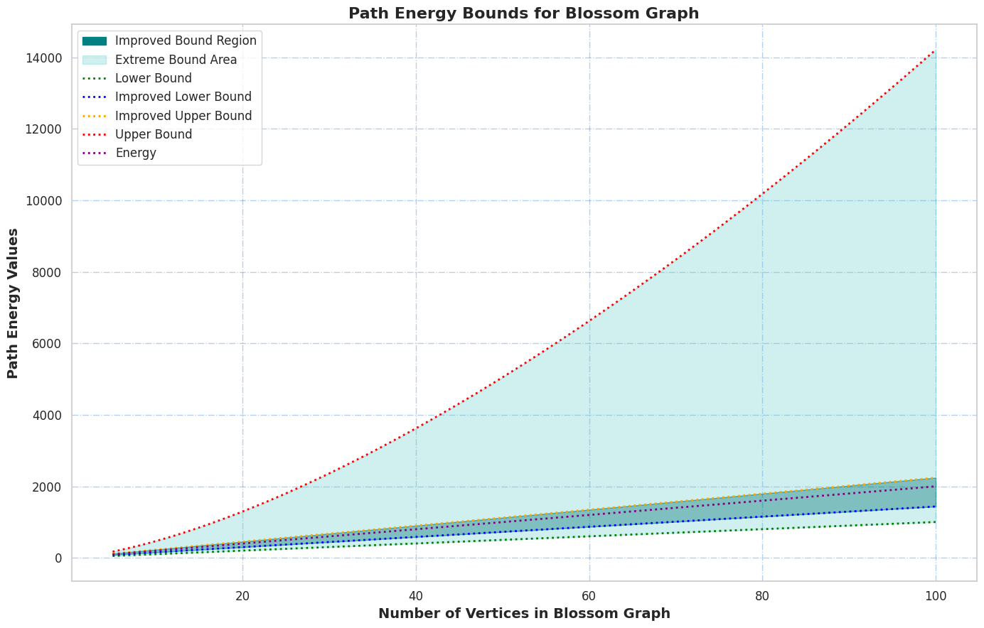
The lower bounds of pathway energy is given by,
\[E_p(Bl_n) \geq \sqrt{5(\varrho_1 + \varrho_2) + \frac{2}{l(l-1)}\prod_{i=1}^{l} (\mu_i^{w_i})^2},\] where \(w_i\) are the weights, \(\sum_{i=1}^{l} w_i = 1\) gives the total sum of the characteristic value weights.
The improved pathway energy lower bound is given by, \[E_p(Bl_n) \geq \sqrt{5(\varrho_1 + \varrho_2) + l(l-1) D^ {\frac{2}{l}}} \quad\text{where} \quad D = |\det A_p(Bl_n)|.\]
Proof. In general, the blossom graph \(Bl_n\) has a vertex-disjoint adjacency matrix of order \(l \times l\), with the number of vertices denoted by \(l = 2n+1\). The characteristic values \(\mu_1, \mu_2, \ldots, \mu_l\) can be determined by solving \(|A_p(Bl_n) – \mu I| = 0\). As similar to the method earlier in Theorem 4.2, the pathway energy \(E_p(Bl_n)\), is the total of the absolute values of these characteristic values.
\([E_p(Bl_n)]^2 = \left(\sum\limits_{i=1}^{l}|\mu_i|\right)^2 + \left(\sum\limits_{i\neq j}|\mu_i| |\mu_j|\right).\)
Case 1: Proof for the pathway energy lower bound of blossom graph
From the Chebyshev’s Inequality (3), we derive that, \[^2 \geq {\sum_{i=1}^{l}|\mu_i|^2 + \frac{2}{l(l-1)} \left( \sum_{i=1}^{l} |\mu_i| \right) \left( \sum_{i=1}^{l} |\mu_i| \right)}.\]
We derive the following from the Weighted AM–GM inequality (4): \[\begin{aligned} {\left[E_p\left(Bl_n\right)\right]^2} &\geq{\sum_{i=1}^{l}|\mu_i|^2 + \frac{2}{l(l-1)} \left( \sum_{i=1}^{l} \mu_i w_i \right) \left( \sum_{i=1}^{l} \mu_i w_i \right)}\quad \text{where} & \sum_{i=1}^{l} w_i = 1, \\ &\geq {\sum_{i=1}^{l}|\mu_i|^2 + \frac{2}{l(l-1)} \prod_{i=1}^{l} \left(\mu_i^{w_i} \right) \prod_{i=1}^{l} \left(\mu_i^{w_i} \right)} \\ &\geq {5(\varrho_1 + \varrho_2) + \frac{2}{l(l-1)} \prod_{i=1}^{l} \left(\mu_i^{w_i} \right)^2}\text { by Theorem 7.1}. \end{aligned}\]
Thus, the lower bound of the pathway energy for blossom graph is,
\(E_p(Bl_n)\geq \sqrt{5(\varrho_1 + \varrho_2)+\frac{2}{l(l-1)} \prod_{i=1}^{l} \left(\mu_i^{w_i} \right)^2}.\)
Case (ii): Proof for the pathway energy improved lower bound.
We obtain that from the AM-GM inequality in Eq. (2). \[\begin{aligned} {\left[E_p\left(Bl_n\right)\right]^2} & =\sum_{i=1}^{l}\left|\mu_i\right|^2+l(l-1) \left|\prod_{i=1}^{l} \left(\mu_i\right)\right|^{\frac{2}{l}} \\ & ={5(\varrho_1 + \varrho_2)+l(l-1) D^{\frac{2}{l}}} \quad { \text {by Theorem 7.1}}.\\ \end{aligned}\]
Thus, the improved lower bound of the pathway energy for blossom graph is, \[E_p(Bl_n)\geq \sqrt{5(\varrho_1 + \varrho_2)+l(l-1) D^{\frac{2}{l}}}.\] ◻
Proof. The Eq. (8) provides a detailed description of the pathway configuration for the vertex-disjoint matrix of the blossom graph. Solving the characteristic equation \((-\mu)^{2n+1}+tr(-\mu)^{2n}+\cdots+det\,A_{p}({Bl}_{n})=0\) derives the \(2n + 1\) characteristic values in this way: \(\mu_1 =\mu_2=\mu_3 =\dots=\mu_{2n} =5 \quad \text{and} \quad \mu_{2n+1} =5(2n)\).
The spectrum can be articulated as: \(\texttt{Spec}\left( \mathbb{A}_p(Bl_n) \right)\) = \(\begin{bmatrix} -5 & 5(2n) \\ 2n & 1 \\ \end{bmatrix}\).
The exact energy path of the blossom graph provided by, \[\begin{aligned} E_p(Bl_n) &= \sum\limits_{i=1}^{2n+1} |\mu_i| =\quad \mid -5 \mid %+\mid -3\mid + \dots +\mid -3 \mid (2n) +5(2n) & = 3(2n-1) + 3(2n-1) \\ =10(2n). \end{aligned}\] The term \(| -5 |\) appears \(2n\) times, while \(5(2n)\) appears once. Consequently, the exact pathway energy bound for the blossom graph is given by: \(E_p(Bl_n) = 10(2n).\) ◻
The upper bound of pathway energy is given by: \(E_p(Bl_n) \leq \sqrt{5l(\varrho_1 + \varrho_2)}\)
The improved upper bound of pathway energy is: \(E_p(Bl_n) \leq \sqrt{5(5(\varrho_1 + \varrho_2))}\).
Proof. This section of the proof establishes the upper bounds using an analogous method of determining characteristic values as in Theorem 4.2.
Case 1: Proof for the path energy upper bound of blossom graph.
For deriving the upper bound Cauchy-Schwarz Inequality (1) leads that, \([E_p(Bl_n)]^2 \leq \left(\sum_{i=1}^{l} \alpha_i \beta_i\right)^2\), where the pathway energy is constrained by the right-hand side. Substituting \(\alpha_i = 1\) and \(\beta_i = |\mu_i|\) leads to the desired conclusion, \[\begin{aligned} \left[E_p(Bl_n)\right]^2 & \leq \left( \sum\limits_{i=1}^{l} 1.|\mu_i|\right)^2 \leq \left( \sum\limits_{i=1}^{l} 1 \right)^2 .\left( \sum\limits_{i=1}^{l} |\mu_i|^2\right) \text {……………………. by (1)}\\ &= 5l(\varrho_1 + \varrho_2) \text {……………………………. by Theorem 7.1}\\ \left[E_p(Bl_n)\right] & \leq \sqrt{5l(\varrho_1 + \varrho_2))}. \end{aligned}\]
Thus, the upper bounds of the pathway energy of the blossom graph concluded by \[E_p(Bl_n)\leq \sqrt{5l(\varrho_1 + \varrho_2)}.\] Case 2: Proof for the pathway energy improved upper bound.
The Weighted Cauchy Schwarz inequality 5 allows us to deduce that, \[\left[E_p(Bl_n)\right]^2 \leq \left( \sum\limits_{i=1}^{l}a_{i}.b_{i}.w_i\right)^2.\]
By substituting \(a_{i}=\frac{1}{(l)^{\frac{3}{2}}}\,|\mu_i|\), \(b_{i}=1\) and \(w_i=\sqrt{5}\), in the above inequality, \[\begin{aligned} \left[E_p(Bl_n)\right]^2 & \leq \left( \sum\limits_{i=1}^{l} \frac{\mu_i^2}{(l)^3}.\sqrt{5}\right) \left( \sum\limits_{i=1}^{l} 1.\sqrt{5}\right)\\ &= 5(5(\varrho_1 + \varrho_2)) \text {…………………….by Theorem 7.1}\\ [E_p(Bl_n)] & \leq \sqrt{5(5(\varrho_1 + \varrho_2))}. \end{aligned}\]
Thus, the improved upper bound of the pathway energy for blossom graph is, \(\left[E_p(Bl_n)\right] \leq \sqrt{5(5(\varrho_1 + \varrho_2))}.\) ◻

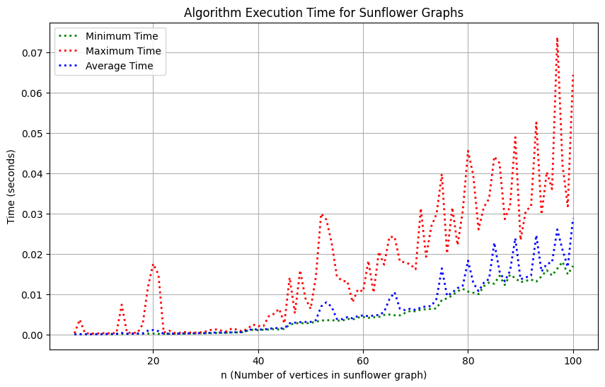
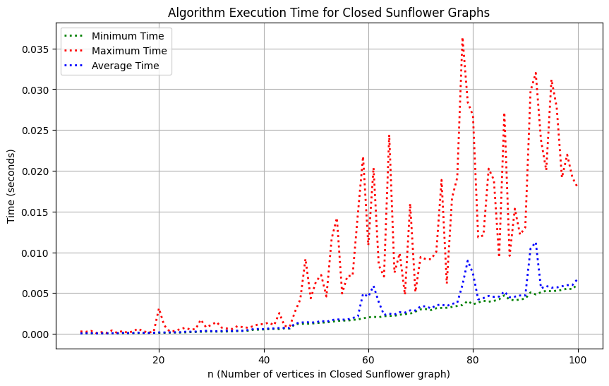
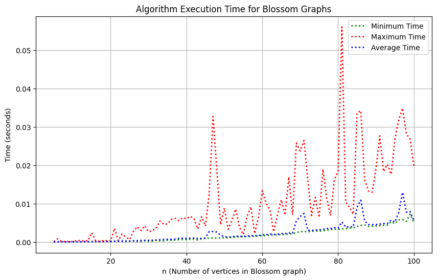
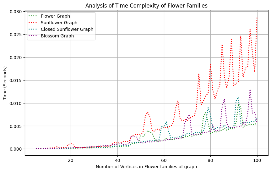
We undertook a comprehensive computational analysis of flower families, employing algorithmic techniques to quantify the energy of these graphs alongside the time taken for each calculation. By plotting energy against computation time, we meticulously assessed the complexity and efficiency inherent in each graph type. Our results reveal that sunflower graphs exhibit a significantly higher complexity compared to the flower families under investigation. Notably, the computational time for sunflower graphs adheres to a complexity of \(O(n^3)\), underscoring its critical nature in relation to the flower families discussed in this study.
This paper presents an innovative algorithmic framework for analyzing pathway energy within flower families, encompassing a wide range of graph types. We established precise limits for pathway energies and conducted an in-depth analysis of time complexity, illuminating significant computational challenges in this domain. The hallmark of our work is the enhanced efficiency and versatility of our pathway energy calculations, providing a robust tool for addressing complex spectral graph problems. These findings pave the way for future research focused on optimizing algorithms and exploring new classes of graphs. Moreover, this research has substantial practical implications for network optimization, improving algorithmic efficiency, and advancing spectral graph theory. Ultimately, our contributions propel the progress of computational graph theory and its related fields.