
Safety management on construction sites for distribution networks is crucial to protect the lives and property of construction personnel. However, some workers lack strong safety awareness, leading to violations of safety regulations, such as disregarding working height and voltage safety distances [5]. Additionally, supervisors often fail to effectively monitor and address potential hazards, resulting in accidents like electric shocks and falls [2]. To mitigate the impact of human factors in safety supervision, video AI detection systems have been explored. However, the relatively open construction sites and distractions, such as passing citizens or obstructed cameras, often trigger false alarms, reducing the reliability of video AI systems and diminishing the effectiveness of supervision [9,3].
This paper presents a pre-control system for ensuring safe behavior in distribution network operations, utilizing LiDAR, gyroscopes, an edge computing module, and a warning module to address distance and altitude detection issues [6]. The edge computing module collects LiDAR point clouds in real time, using point cloud aggregation technology and tracking algorithms for object recognition. Spatial distance measurement technology is employed to identify operators, the ground, distribution network areas, and high-voltage equipment, while also measuring operating height and spatial distances. Dangerous behaviors during operations trigger reminders to alert workers, ensuring safer operations and preventing accidents [8].
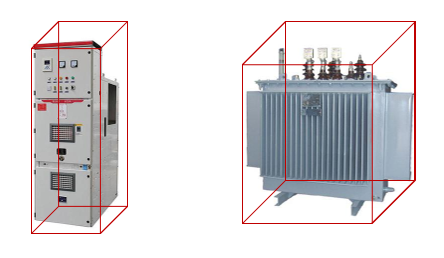
The pre-control device for ensuring safe operation behavior in distribution network scenarios consists of seven modules: LiDAR module, tripod support module, gyroscope, edge computing module, battery-powered module, configuration and debugging tablet, and early warning module. The LiDAR module, gyroscope, edge computing module, tripod, and battery-powered module form the core of the pre-control device, with the external battery connected via aviation quick connectors (see Figures 1, 2, and 3).
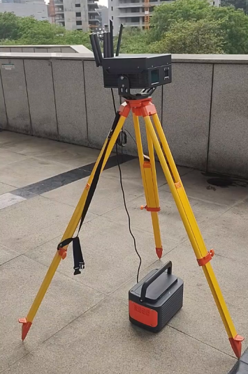
The edge computing module connects directly to the LiDAR via a network port and the gyroscope via the RS232 serial port. It is also linked to the early warning module and debugging tablet through shared Wi-Fi, enabling seamless data transmission for data collection, scene configuration, and alarm message communication [14,13]. The edge computing module serves as both the bridge and the brain of the device, responsible for point cloud collection, storage, target recognition, distance measurement, and controlling the early warning module for operator alerts.
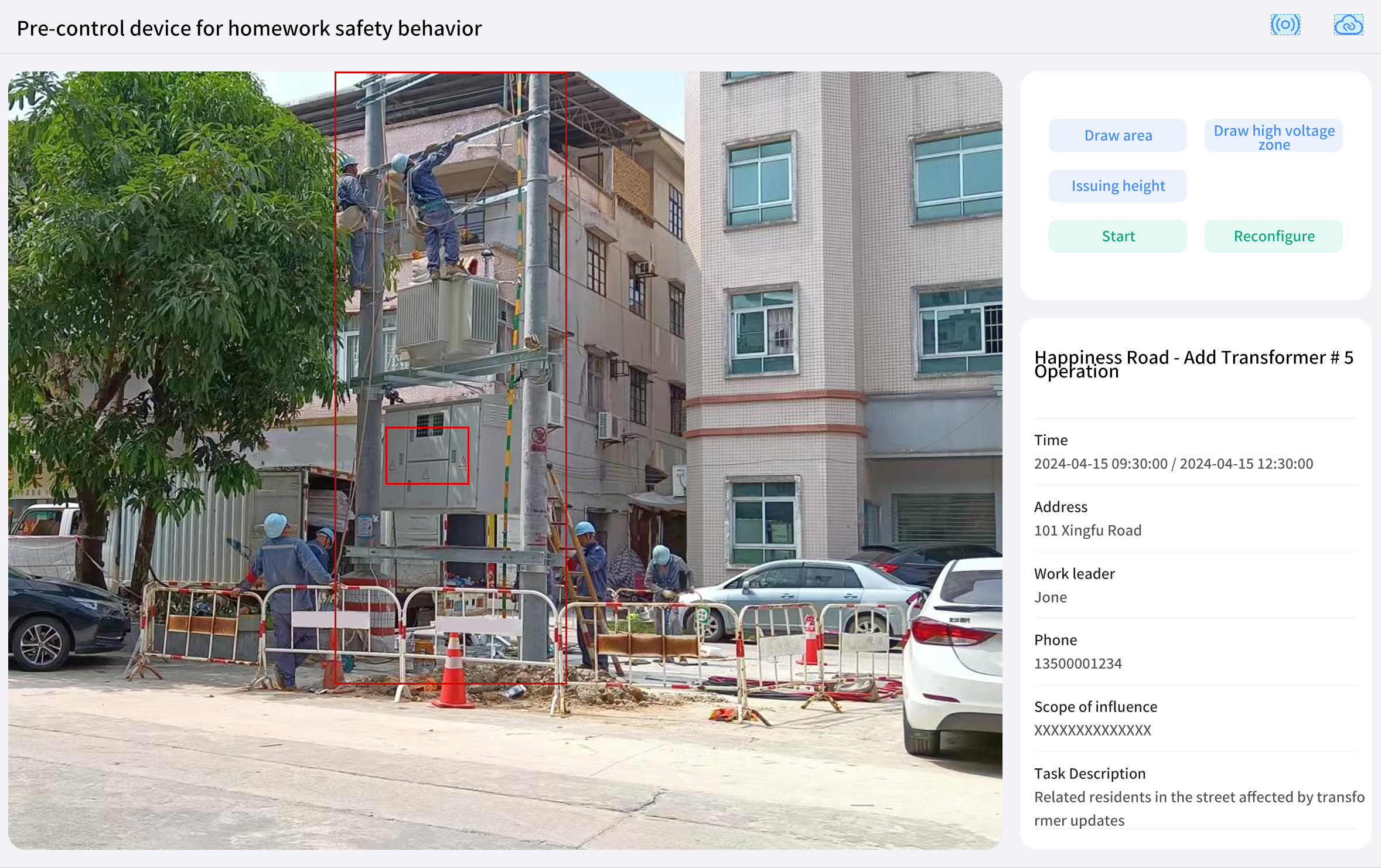
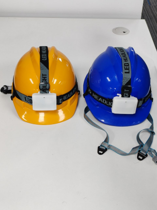
Operators and work leaders, equipped with safety helmets containing early warning modules, receive timely alerts from the device. The pre-control device calculates the operator’s ground clearance and the spatial distance from high-voltage equipment. If the clearance exceeds 2 meters, the edge computing module triggers the early warning module to remind the operator to wear a seatbelt when working at height. If the spatial distance from high-voltage equipment falls below the safety threshold, the module alerts the operator to the potential shock hazard [1, 11]. If there is significant obstruction in the LiDAR’s view for more than 3 seconds, the early warning module alerts the station’s control personnel.
The performance requirements of the system are summarized in Table 1.
| Laser Band | 905nm |
| Laser Class | Level 1 (Eye Safe) |
| Laser Channel | 144 lines |
| Measuring Range | 190m at 10% reflectivity |
| Ranging Accuracy | \(\pm\) 2cm |
| Single-return Data Rate | 240,000 points/s (single echo), 480,000 points/s (double echo), 720,000 points/s (triple echo) |
| Field of View | Vertical 77.2\(^\circ\), Horizontal 70.4\(^\circ\) |
| Angular Resolution | 0.03\(^\circ\) horizontally, 0.28\(^\circ\) vertically |
| Image Resolution | 1200W (3840*2880) |
| Sensor Type | 1/2.3″ Progressive Scan CMOS |
| Minimum Illumination | Color 0.01 Lux @(F1.2, AGC ON) |
| Dynamic Range | 72db |
| Lens | 4.3 mm, F2.0 |
| Field of View (Lens) | 98\(^\circ\) Horizontal, 82.8\(^\circ\) Vertical, 45.1\(^\circ\) Vertical, 98\(^\circ\) Diagonal |
| Angle Adjustment | Manual: Tilt 0\(^\circ\), 15\(^\circ\), 25\(^\circ\), 35\(^\circ\), Electric: Pitch -45\(^\circ\)-45\(^\circ\), Horizontal 0-360\(^\circ\) |
| Gateway Performance | CPU: 4 cores and 8 threads, frequency 2.8-4.70 GHz, memory: 16GB, hard disk: 1TB M.2 |
| Gyroscope | Two-axis gyroscope |
| Satellite Positioning | Beidou, GPS |
| Wi-Fi Sharing | 802.11 (a/b/g/n/ac), dual-band 2.4G+5.8G |
| Mobile Communication | 5G, backward compatible with 4G |
| SIM Card | Nano-SIM |
| Events | Operation safety distance detection, cross-regional operation detection, and helmet wearing detection |
| Alarm Linkage | Helmet alarm (sound, vibration, light), on-site tablet alarm, alarm message reporting platform |
| Interface | 15-pin waterproof quick connector *1, RJ45 waterproof quick connector *1 |
| Button | Waterproof power button |
| Power Supply | DC12V |
| Power Consumption | Terminal: \(\leq\)75W, Gimbal: \(\leq\)5W, Motion: \(\leq\)50W |
| Alarm Size | 200mm (Length) x 120mm (Height) x 220mm (Depth) |
| Terminal Size | 60mm (Length) x 50mm (Height) x 20mm (Depth) |
| Weight | Terminal: 4.0kg, Gimbal: 3.5kg |
In 3D data processing and robot vision, aligning point clouds with the direction of gravity is a crucial task. It helps reduce the complexity of data processing and improves the performance of subsequent algorithms (see Figures 4 and 5).
Obtaining IMU Data
First, data must be acquired from the IMU (Inertial Measurement Unit). IMUs typically contain sensors such as accelerometers and gyroscopes. Accelerometers measure the acceleration of an object in three directions, including the acceleration component generated by gravity [7].
Estimating the Direction of Gravity
When the IMU is at rest or near stationary, the output of the accelerometer mainly reflects the effect of gravity. The gravitational acceleration component is extracted using filtering algorithms (such as Kalman filter, complementary filter, etc.), resulting in a three-dimensional vector representation of the gravity direction.
Point Cloud Preprocessing
Before aligning the point cloud with the direction of gravity, preprocessing is required. This may involve filtering, downsampling, denoising, etc., to reduce redundant information and noise in the point cloud, improving the accuracy and efficiency of subsequent processing [10].
Aligning the Point Cloud with the Direction of Gravity
Aligning the point cloud with the direction of gravity involves a coordinate transformation. The specific steps are as follows:
Calculate Rotation Matrix: Compute a rotation matrix that transforms the point cloud from the original coordinate system to the reference coordinate system. The rotation matrix can be obtained using quaternion, Euler angles, or directional cosine matrices. The estimated gravity direction vector is used to calculate the rotation matrix.
Apply Rotation Matrix: Apply the rotation matrix to each point in the point cloud, transforming it from the original coordinate system to the reference coordinate system. In this way, each point in the point cloud will be aligned with the direction of gravity.
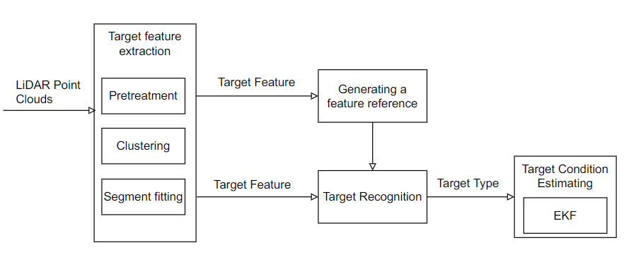
The point cloud segmentation algorithm based on the adaptive distance threshold uses multi-feature matching to achieve target recognition. The extended Kalman filter (EKF), based on the Constant Turn Rate and Acceleration (CTRA) model, is employed to update and associate the target state, thereby reducing the impact of missed detections on target tracking [12]. The overall flow of the method is shown in Figure 6.
Point cloud segmentation based on the distance threshold can be expressed as:
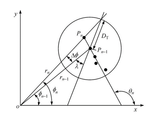
\[\label{e1} {\text{d}}(P_{n-1},P_n) > d_{\text{th}}, \tag{1}\] where \({\text{d}}(P_{n-1}, P_n)\) represents the distance between two adjacent points in the original point cloud, which is the distance threshold. In general, the greater the distance between the target and the sensor, the larger the distance between adjacent points on the target surface, due to the fixed angular resolution of the LiDAR, as shown in Figure 7. The distance threshold is related to the radial distance of the point and can be expressed as:
\[\label{e2} d_{\text{th}} = r_{n-1} \frac{\sin (\Delta \varphi)}{\sin (\lambda – \Delta \varphi)} + \varepsilon, \tag{2}\] where \(r_{n-1}\) is the radial distance of the point \(p_{n-1}\), \(\Delta \varphi\) is the angular resolution of the LiDAR, \(\lambda\) is the angular threshold used to calculate the maximum spacing, and \(\varepsilon\) is the sensor error.
However, using the above clustering algorithm, point clouds located on surfaces that are relatively parallel or perpendicular to the direction of the laser pulse on the same target may not be segmented into the same target. To improve this, \(|\alpha – \beta|\) is used to represent the relative relationship between the positions of two adjacent points and the laser beam. If \(|\alpha – \beta|\) is less than the set angular threshold, and \(\lambda\) is considered such that the two points are on a surface relatively perpendicular to the laser beam, a larger value of \(\lambda\) is set to obtain a smaller \(d_{\text{th}}\) distance threshold. If \(|\alpha – \beta|\) is greater than the set angular threshold, a smaller \(d_{\text{th}}\) is set to obtain a larger \(\lambda\) distance threshold.
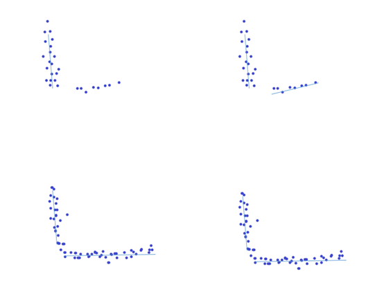
The line segment fitting is performed using the endpoint iterative fitting algorithm (Itratif, Endpointfitting, Pu) on each point cloud cluster after clustering. This method connects the first and last data points in each point cloud cluster to form a line segment by calculating the maximum distance of other data points from this line segment. If the maximum distance exceeds the set threshold, the line segment is divided into two line segments at the data point corresponding to the maximum distance. This check is repeated until all line segments in the point cloud cluster no longer require division [4].
In the actual operating environment, occlusion of the target part may affect the clustering of point clouds, causing the data points of the same target to be divided into two point cloud clusters. In this paper, the merging of point cloud clusters is completed by comparing the spacing between the clusters and the slope of their line segments. As shown in Figure 8, the upper human target is occluded, and the corresponding point cloud is divided into two parts. The last data point of the point cloud cluster on the left side of the target is connected with the first data point of the point cloud cluster on the right to form a line segment. If the distance of the line segment is less than the set distance threshold, and the difference between the slope of the left and right point cloud clusters is less than the set slope threshold, the two point clouds are merged, and the line segment is refitted.
After point cloud clustering and line segment fitting, the operator target can be represented by one line segment, the machine by two line segments, and the vehicle by two line segments. The following characteristics are defined:
The length of the line segment for a single segment target.
\({I_1}, {I_2}\), representing the lengths of the two line segments for a two-segment target.
\({\operatorname{var}_r}\) represents the distance variance of the point cloud cluster.
A large number of point cloud data are collected and processed according to the above method, with each target category manually labeled. The feature reference intervals of different types of targets can be obtained, and target type identification can be achieved by comparing the feature set of an unknown target with the generated reference intervals for each type of target.
For the detected target at each moment, it is necessary to associate it with the historical target in order to filter the target state. The Extended Kalman Filter (EKF), based on the Constant Turn Rate and Acceleration (CTRA) model, is used to predict the target state:
\[\label{e3} \mathbf{x}_{k}^{-} = \mathbf{A} \mathbf{x}_{k-1}. \tag{3}\]
The system state is \({\{ x, y, a, v, \alpha \} ^T}\), which successively represents the lateral distance, longitudinal distance, velocity direction, velocity, and acceleration of the target in the coordinate system of the pre-control device. Here, \(\mathbf{A}\) is the state transfer matrix. The speed of the pre-control device and the heading angular velocity are measured and provided as input to the filter as control quantities.
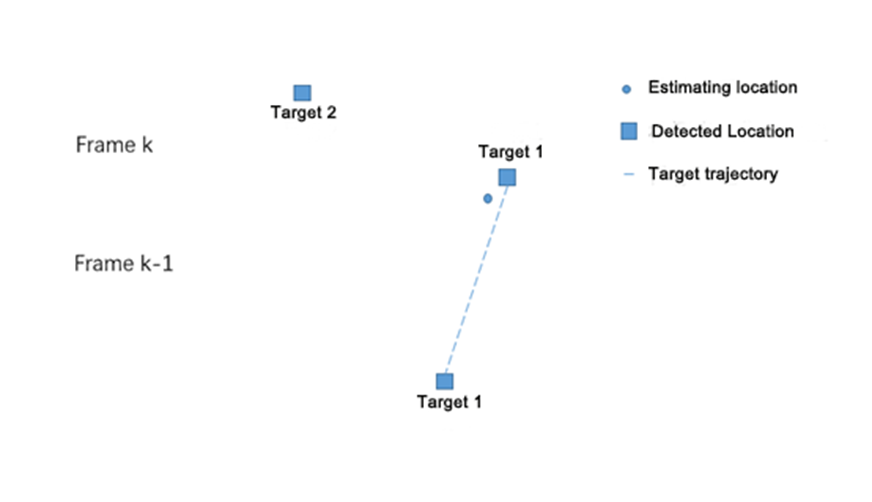
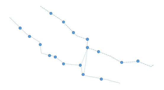
As shown in Figure 9, the target state at time \(k\) is predicted based on the target information at time \(k-1\). There are two measurement targets at time \(k\). If the Euclidean distance between the calculated and estimated position of current target 1 is less than the set distance threshold, the corresponding target is associated with the target at time \(k-1\) and identified as the same target. The target measurement is then used to update the target state. For new targets that are not associated with existing targets, the system state and the related error matrix of the Kalman filter are initialized and expanded, which is used to predict the target state and target association at the next moment. If a historical target is not associated with the target at the current time, state estimation will continue to be performed using the information from the previous time until the continuous unassociated time exceeds the set threshold, at which point the target is eliminated.
The construction of the Oriented Bounding Box (OBB) requires first determining a suitable direction. The average of the coordinates of all vertices of the target object is calculated, which serves as the center of the OBB cube’s bounding box. Next, the covariance matrix is constructed, and the eigenvalues and corresponding eigenvectors are obtained to construct the OBB bounding box. The specific process is as follows:
\[\label{e4} m = \frac{1}{3n} \sum_{i=1}^{n} \left( a^i + b^i + c^i \right), \tag{4}\] where \(a^i\), \(b^i\), and \(c^i\) represent the 3 vertices of the \(i\)-th triangle of the target object, and \(n\) is the number of vertices.
The covariance matrix \(M\) is constructed from the mean value: \[\label{e5} M_{jk} = \frac{1}{3n} \sum_{i=1}^{n} \left( \overrightarrow{a_{\jmath}^l a_k^l} + \overrightarrow{a_{\jmath}^l a_k^l} + \overrightarrow{a_{\jmath}^l a_k^l} \right), \quad 1 \leq \mathrm{j}, \mathrm{k} \leq 3. \tag{5}\]
As shown in Figure 10, the eigenvalues and corresponding eigenvectors of the matrix \(M\) are solved. The eigenvectors are normalized and used as the three coordinate axes of the OBB cube bounding box. Finally, the target object is projected along the three coordinate axes, and the OBB cube bounding box is constructed according to the maximum and minimum values of the projection distances. Figure 10 illustrates the OBB envelope box for both the bike and bust models.
Based on the point cloud data of the reference coordinate system after leveling, the operator’s point cloud is extracted through point cloud clustering, line segment fitting, and target recognition. The target object frame is selected using the 3D cube bounding box, and the center point coordinates of the bounding box are taken. The distance between the center point and the LiDAR, along with the angle \(\angle 1\) with the horizontal plane, are calculated through the XYZ values. \(H_1\) is calculated using the Pythagorean theorem, and the height of the operator \(H\) is set to \(H_2\) at the center point of the LiDAR of the pre-control device: \[H = H_1 + H_2 = C_1 \cdot \sin(\angle 1) + H_2.\]
As shown in Figure 11, through target recognition training, high-voltage equipment such as distribution network stations, transformers, transformer terminals, high-voltage drop-out fuses, high-voltage arresters, and high-voltage down conductors are identified. Before the operation, the scene of the station area is initialized, and the point cloud of the operation area is collected. The identified high-voltage equipment is selected, and the coordinate subset of the edge points of the aggregate point cloud (reference point cloud) for each high-voltage device is extracted, allowing for voltage safety distance calibration. When the operator enters the station area, the recognition algorithm identifies the operator and tracks it. The distance between the edge point cloud of the comparison point cloud and the edge point coordinates of the calibrated high-voltage equipment aggregation point cloud (reference point cloud) is calculated. The nearest neighbor distance from each point cloud in the comparison point cloud to the reference point cloud is also calculated. The octree structure can be used to improve the search rate of neighborhood point clouds.
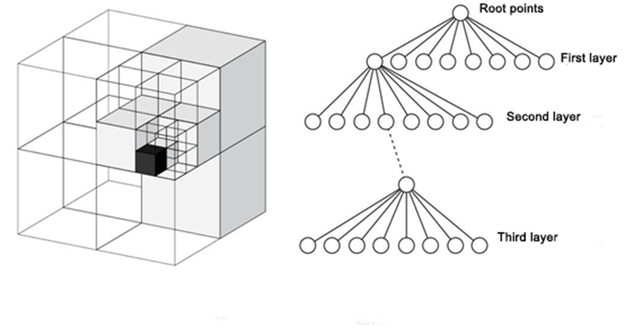
An octree is a tree-like data structure used to describe 3D space and is most commonly used to divide three-dimensional space. The octree subdivision divides the cube containing the point cloud into 8 equivalent subcubes, and each subcube undergoes this recursive partitioning process (see Figure 12) until the set octree depth is reached.
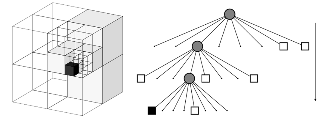
An octree structure is a form of data list that encodes the absolute positions of points at all subdivision levels and is suitable for spatial indexing. Two points within the same cell at a given subdivision level have the same (partial) association code. The code consists of a 3-bit (0-7) set (see Figure 13), representing the relative position on each subdivision level cell. This allows for fast binary search and point cloud space scanning by sorting the code, making octree structure coding more efficient, and enabling quick searching of all points in a code or set.
The distance between two 3D coordinate points can be calculated using the Euclidean distance formula. Suppose that the reference point cloud \(P_1\) and the comparison point cloud \(P_2\) in 3D space have coordinates \(P_1(x_1, y_1, z_1)\) and \(P_2(x_2, y_2, z_2)\), respectively. Then, the distance between the two points can be calculated by the following steps:
Calculate the square of the difference on each coordinate axis: First, calculate the difference between the coordinate values of the two points on the X, Y, and Z axes, and square these differences respectively. This means calculating \((x_2 – x_1)^2\), \((y_2 – y_1)^2\), and \((z_2 – z_1)^2\).
Sum: Add the sum of the three squares obtained above, i.e., \((x_2 – x_1)^2 + (y_2 – y_1)^2 + (z_2 – z_1)^2\).
Square Root: Finally, take the square root of the sum from the previous step: \[\sqrt{(x_2 – x_1)^2 + (y_2 – y_1)^2 + (z_2 – z_1)^2},\] which gives the straight-line distance between the two points.
This calculation formula is based on the generalization of the Pythagorean theorem in three-dimensional space and applies to any two points in three-dimensional space, regardless of their position.
The operation of the distribution network station area in a certain area was taken as the experimental object (see Figure 14).
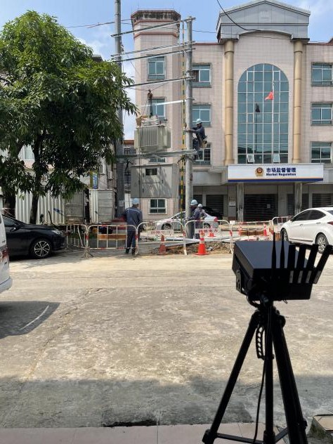
The device is used to detect the distribution network operation area, and the identification ability of the device is analyzed through the algorithm detection results.
According to the truth value and the target recognition results, the above indexes are obtained and compared with a feature-based target recognition method. The comparison of various target recognition results is shown in Table 2. Compared with the methods in the references, the proposed method can provide more accurate and reliable target recognition results for the three types of targets. Overall, the recognition accuracy of the proposed method is improved by 3.5%, and the recall rate is increased by 5.8%.
| Target category | Target Numbers | TPS | FPS | FNS | P (%) | R (%) | TPS | FPS | FNS | P (%) | R (%) |
| Personnel | 105 | 100 | 3 | 5 | 97.1 | 95.2 | 92 | 15 | 13 | 86.0 | 87.6 |
| Equipment | 152 | 131 | 24 | 21 | 84.5 | 86.2 | 122 | 27 | 30 | 81.9 | 80.2 |
| Vehicle | 187 | 147 | 35 | 40 | 86.8 | 78.6 | 138 | 53 | 49 | 72.3 | 73.8 |
| All targets | 444 | 378 | 62 | 66 | 85.9 | 85.1 | 352 | 75 | 92 | 82.4 | 79.3 |
According to the surface of the device detection and on-site manual measurement results, the detection deviation of the personnel working height is kept within 10 cm. The surface of the device detection and on-site manual measurement results are shown in Table 3.
| Status | Device detection (cm) | Manual measurements (cm) | Deviation (cm) | |
| The first time | Standing erect | 245 | 249 | 4 |
| The second time | Standing erect | 368 | 360 | 8 |
| The third time | Standing erect | 233 | 230 | 3 |
| The fourth time | Standing erect | 254 | 258 | 4 |
| The fifth time | Standing erect | 274 | 271 | 3 |
| The sixth time | Stooping | 243 | 248 | 5 |
| The seventh time | Stooping | 258 | 252 | 6 |
| The eighth time | Stooping | 301 | 296 | 5 |
| The ninth time | Stooping | 266 | 264 | 2 |
| The tenth time | Stooping | 272 | 275 | 3 |
According to the spatial distance detection function between the operator and the high-voltage equipment, the detection deviation of the spatial distance between the operator and the high-voltage equipment is kept within 5 cm based on the surface of the device detection and on-site manual measurement results for the 10 test results (see Table 4).
| Device detection (cm) | Manual measurements (cm) | Deviation (cm) | |
| The first time | 68 | 69 | 1 |
| The second time | 69 | 68 | 1 |
| The third time | 65 | 67 | 2 |
| The fourth time | 60 | 62 | 2 |
| The fifth time | 64 | 65 | 1 |
| The sixth time | 69 | 65 | 4 |
| The seventh time | 67 | 68 | 1 |
| The eighth time | 66 | 65 | 1 |
| The ninth time | 63 | 62 | 1 |
| The tenth time | 60 | 63 | 2 |
Distribution network operation safety accidents can lead to personal injuries, economic losses for enterprises, and, in the case of major accidents, pose a threat to public safety, cause public panic, and affect social stability, resulting in significant social harm and impact. However, there are currently very few distribution network operation safety control devices in use. The operation safety control device designed in this paper provides more accurate prompts and comprehensive protection for distribution network operators. At the same time, it has characteristics such as intelligence, convenience, stability, reliability, economic viability, and environmental protection. It is highly applicable and aligns with current development trends, as well as the safety needs of distribution network operations. The device boasts a high degree of integration, with simple deployment, and can be widely used in environments such as transmission hanging lines, distribution network hanging lines, distribution network station areas, substations, booster stations, converter stations, and high-voltage operating environments like power plant switchyards. It can monitor external damage behaviors and operational safety behaviors, such as mechanical construction, personnel operation, and temporary construction. This helps to prevent electric shock accidents and effectively protect the operational safety of transmission lines and high-voltage main equipment.