
With the rapid development of information technology such as artificial intelligence, internet of things, big data and so on, intelligent manufacturing has gradually become the direction of manufacturing upgrading. In the field of intelligent manufacturing, machine vision technology, as one of the important technical means, is being widely used [6,8,13]. Machine vision technology refers to the processing and analysis of images or videos through computers and related hardware systems, so that they have the visual ability of the human eye, thus achieving the recognition, detection, measurement, tracking and other functions of the object [26,9,23]. Machine vision technology can process images, videos and other types of data, the core of this technology is image processing algorithms and pattern recognition algorithms, which play an important role in the automated detection of precision components [11,1,24].
Machine vision technology can be used for automated inspection and quality control of precision components on production lines. For example, in the process of automobile manufacturing, the application of machine vision can detect whether the size of the components meets the standard, and whether the components and the whole vehicle are properly spliced together [7,17,29]. At the same time in the detection, machine vision can also collect and analyse the data to help enterprises timely find the problems on the production line, and make improvements. In intelligent manufacturing, machine vision technology features and application advantages can improve the quality and efficiency of precision components, achieve intelligent production, and play an important role in enhancing the core competitiveness of enterprises [4,27,22,16].
Literature [10] explores the many applications of machine vision and the role it plays in Industry 4.0 and presents various smart technologies in the form of diagrams and charts of machine vision for Industry 4.0. It is indicated that any step in Industry 4.0 and related digital industrial transformation, including manufacturing, supply chain, etc., reflects different innovative approaches. Literature [20] developed an image-based framework which uses pre-trained CNNs and ResNet-101 to detect defects, and confirmed the feasibility of the framework by launching a study on common surface defects in centre polishing. In addition, ResNet-101 is used to extract features and combined with SVM as a classifier to detect defective images, and the results show that the proposed framework effectively performs image classification with 100% detection accuracy. Literature [2] proposes a machine vision model which is capable of identifying the defects of a product and modifying it to obtain a perfect product, which meets the requirements of ensuring product quality in the context of Industry 4.0. Literature [12] analysed the application of machine vision systems in the automotive industry China in recent years and predicted the trend of the future development of this technology. The results of their analyses show that machine vision technology is more often used in quality-related tasks and has shown excellent results in the automotive manufacturing sector. Literature [28] shows that computer vision technologies have promoted the informatisation, digitisation and intelligence of industrial manufacturing systems, and based on the rapid development of CV technologies, a comprehensive review of the current status of the development of these technologies as well as their applications in manufacturing is presented. Literature [14] introduced the current development of machine vision technologies in terms of hardware, software and industrial inspection, indicated that the combination of multiple technologies can promote the performance and efficiency of inspection in various applications, and affirmed the development potential of machine vision systems in industry. Literature [5] presents the results of a study that investigated the effect of lighting technology on machine vision inspection techniques for automated assembly machines with highly reflective metal surfaces. Whereas the light reflection from the machine surface makes glare in the image a major difficulty, inspections were carried out using a high resolution high-speed camera under different lighting conditions with the aim of checking the effect of illumination on the inspection performance of flat specular reflections.
The article builds a binocular stereo vision system, measures the dimensions of precision components by using the method of dual camera calibration, and then uses BP neural network and genetic algorithm to calibrate the camera. The edge detection algorithm and Hough transform algorithm are used to process the images of precision components and identify them, so as to construct a precision component detection model based on machine vision. The model is applied to the detection of bearing components to detect and analyse the dimensions, edges, and geometric parameters of the bearing components and identify the loose bearing components. Finally, the false detection rate and leakage rate of this paper’s precision component detection model are tested under six angles to examine the adaptability of this paper’s model to the detection angle.
The binocular stereo vision system is shown in Figure 1, assuming that the orthogonal unit matrices and translation vectors of the outer parameters of the two cameras are \(R_{1} ,t_{1} ,R_{2}\) and \(t_{2}\), respectively, indicating the transformation relationship between the world coordinate system \(C_{w}\) relative to the camera coordinate system \(C_{1}\) and the camera coordinate system \(C_{2}\). If a point \(P\) in space, it is in the world coordinate system and the two camera coordinate system under the coordinates of \(X_{w} ,X_{c1}\) and \(X_{c2}\), respectively, then the coordinate transformation can be obtained: \[\label{GrindEQ__1_} X_{C1} =R_{1} X_{w} +t_{1} , \tag{1}\] \[\label{GrindEQ__2_} X_{C2} =R_{2} X_{w} +t_{2} . \tag{2}\]
Eliminating the coordinates of point \(P\) in Eqs. (1) and (2) in the world coordinate system \(X_{w}\), the relative positional relationship between the two cameras in the binocular vision system can be expressed as: \[\label{GrindEQ__3_} X_{C1} =RX_{C2} +t . \tag{3}\]
In the formula, \(R=R_{1} R_{2}^{-1} ,t=t_{1} -R_{2}^{-1} t_{2}\).
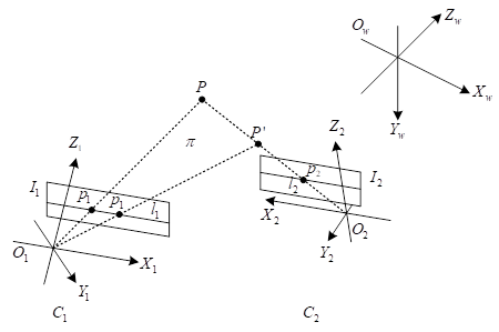
Let the chi-square coordinate of spatial point \(P\) in the world coordinate system be \(X_{p} =[X_{wp} ,Y_{wp} ,Z_{wp} ,1]^{T}\), denoted as \(x_{p} =[x^{{}_{T} } ,1]^{{}_{T} }\), where \(x=[X_{wp} ,Y_{wp} ,Z_{wp} ]^{T}\). The chi-square coordinates of image points \(p_{1}\) and \(p_{2}\) of spatial point \(P\) projected onto the image planes of the left and right cameras of the binocular vision system, \(I_{1}\) and \(I_{2}\), are \(u_{1}\) and \(u_{2}\), respectively, and can be obtained by denoting the projection matrices of the two cameras, \(M_{1}\) and \(M_{2}\), with the \(3\times 3\) part of the left part denoted as \(M_{i1} (i=1,2)\), and the \(3\times 1\) part of the right part denoted as \(m_{i} (i=1,2)\): \[\label{GrindEQ__4_} Z_{c1} u_{1} =M_{11} x+m_{1} , \tag{4}\] \[\label{GrindEQ__5_} Z_{c2} u_{2} =M_{21} x+m_{2} , \tag{5}\] where \(Z_{c1}\) and \(Z_{c2}\) are the coordinates of the space point \(P\) in the direction of the camera coordinate system \(Z_{c}\), which can be obtained by collating Eq. (4) and Eq. (5): \[\label{GrindEQ__6_} Z_{c2} u_{2} -Z_{c1} M_{21} M_{11}^{-1} u_{1} =m_{2} -M_{21} M_{11}^{-1} m_{1} . \tag{6}\]
Denote the vector on the right-hand side of Eq. (6) as \(m\), i.e: \[\label{GrindEQ__7_} m=m_{2} -M_{2} M_{1}^{-1} m_{1} . \tag{7}\]
Assume vector \(m=[m_{x} ,m_{y} ,m_{z} ]^{T}\), which has an antisymmetric matrix of \([m]_{x}\), i.e: \[\label{GrindEQ__8_} [m]_{x} =\left[\begin{array}{ccc} {0} & {-m_{z} } & {m_{y} } \\ {m_{z} } & {0} & {-m_{x} } \\ {-m_{y} } & {m_{x} } & {0} \end{array}\right] . \tag{8}\]
By the nature of antisymmetric matrix, i.e. \([m]_{x} m=0^{T}\), it is obtained from Eq. (6): \[\label{GrindEQ__9_} [m]_{\times } (Z_{c2} u_{2} -Z_{c1} M_{21} M_{11}^{-1} u_{1} )=0^{T} , \tag{9}\] where \(0^{T} =[\begin{array}{ccc} {0} & {0} & {0} \end{array}]^{T}\), is obtained by dividing both sides of Eq. (9) by \(Z_{c2}\) at the same time and noting \(Z_{c} =\frac{Z_{c1} }{Z_{c2} }\): \[\label{GrindEQ__10_} [m]_{\times } Z_{c} M_{21} M_{11}^{-1} u_{1} =[m]_{\times } u_{2} . \tag{10}\]
The right vector \([m]_{\times } u_{2} =m\times u_{2}\) of Eq. (10) is orthogonal to \(u_{2}\). The positional relationship between the two cameras in the binocular stereo vision system can be obtained by multiplying \(u_{2}^{{\rm \overline{\scriptstyle\,|} }}\) by both sides of the above equation on the left and dividing both sides of the resultant equation by \(Z_{c}\) at the same time: \[\label{GrindEQ__11_} u_{2}^{{\rm \overline{\scriptstyle\,|} }} [m]_{\times } M_{2} M_{1}^{-1} \mu _{1} =0^{{\rm \overline{\scriptstyle\,|} }} , \tag{11}\] where \([m]_{\times } M_{21} M_{11}^{-1}\) is the fundamental matrix, determined by the relative positions of the two cameras in the stereo vision system.
In binocular vision system, if the chi-square coordinate of image point \(p_{1}\) is known to be \(u_{1}\), the polar equation on the image plane of \(I_{2}\) can be obtained from Eq. (11) \(l_{2}\). Similarly, if the secondary coordinates \(u_{2}\) of the image point \(p_{2}\) are known, the equation \(l_{1}\) of the polar line in the \(I_{1}\) image plane corresponding to the point \(p_{2}\) can be found from Eq. (11). In a stereo vision system, assuming that a point P in space is projected on the image plane \(I_{1}\) and \(I_{2}\) the chi-square coordinates of image points \(p_{1}\) and \(p_{2}\) are (507.7341, 324.2181, 1.0000), (452.3865, 380.6996, 1.0000), respectively, and from Eq. (11), we can obtain the following: The corresponding polar line \(l_{2}\) of point \(p_{1}\) is -3.4942\(u\)-1.8063\(v\)+2.35983\(\times\)10\({}^{3}\)=0. The corresponding polar line \(l_{1}\) of point \(p_{2}\) is 3.4626\(u\)+1.9127\(v\)-2.29463\(\times\)10\({}^{3}\)=0.
On the other hand, if any point \(p_{2}\) on the image plane \(I_{2}\) is known, only the polar line \(l_{2}\) corresponding to it can be found, while the chi-square coordinates of its corresponding point \(p_{1} {}^{'}\) on \(I_{1}\) cannot be uniquely determined. To obtain the coordinates of the corresponding point \(p_{1} {}^{'}\), as shown in Figure 1, it is also necessary to know the position of the spatial point P’ on the O\({}_{2}\)P line. Substituting the corresponding chi-square coordinates obtained above and the fundamental matrix of the system into Eq. (11) yields \(u_{2} {}^{T} [m]_{\times } M_{21} M_{11} {}^{-1} u_{1} =7.4829\times 10^{-4}\), which basically satisfies the constraints.
For the measurement of top surface, bottom surface and side surface, the accuracy is required to be within 30\(\mu\)m, and it is difficult to achieve micron-level measurement accuracy by a single camera. Taking the top surface measurement as an example, assuming that the single edge error of edge detection can be controlled within 5 pixels, when a single camera is selected to collect the global image of the top surface circle, in order to ensure the measurement accuracy, the camera’s single-pixel accuracy must be at least less than 2 \(\mu\)m in order to meet the requirements. If the diameter of the top surface circle is 80mm, then the field of view of the camera is at least 80 \(\mathrm{\times}\) 80mm². Single-pixel accuracy of 2\(\mu\)m, horizontal and vertical resolution of at least 80,000\(\mu\)m / 2\(\mu\)m = 40000, can be introduced to the camera resolution of at least 40,000 \(\mathrm{\times}\) 40,000 = 160,000,000, i.e., theoretically, if you want to meet the measurement accuracy, at least 1,600,000,000 resolution of the camera, but the use of such a camera is obviously unrealistic.
Through the above analysis, for large-size high-precision measurement, using a single camera is difficult to achieve, need to seek other solutions. How to make the camera resolution in a certain size, effectively improve the single-pixel accuracy is a problem that needs to be solved. It is considered that the camera field of view can be reduced, i.e., instead of using a single camera to capture the global image, two cameras are used to capture the local image separately, so that the distance value from the edge to the optical centre can be obtained. However, the global size measurement task cannot be accomplished by the information from the local images alone, so the positions of the two cameras are calibrated to obtain the distance value between the photocentres of the two cameras, and this value is added to the edge-to-centre distances of the two edges to achieve the global size measurement.
Camera perspective model
The camera perspective model is shown in Figure 2, with \(O_{1} XY\) being the image coordinate system expressed in physical units and \(OUV\) being the image in pixels.
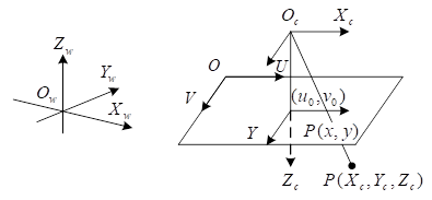
\(O_{w} X_{w} Y_{w} Z_{w}\) and \(O_{c} X_{c} Y_{c} Z_{c}\) are the world coordinate system and the camera coordinate system expressed in physical units, respectively. Assuming that the chi-square coordinates of a spatial point \(P\) in the world coordinate system and the camera coordinate system are \((X_{w} ,Y_{w} ,Z_{w} ,1)\) and \((X_{c} ,Y_{c} ,Z_{c} ,1)\), respectively, and the chi-square coordinates of the feature point projected to the image plane point \(P\) are \((x,y,1)\) and \((u,\nu ,1)\), respectively, then the perspective transformation relationship of the camera can be expressed as follows: \[\begin{aligned} \label{GrindEQ__12_} Z_{e} \left[\begin{array}{c} {u} \\ {\nu } \\ {1} \end{array}\right]&=\left[\begin{array}{cccc} {a_{a} } & {s} & {u_{0} } & {0} \\ {0} & {a_{\nu } } & {\nu _{0} } & {0} \\ {0} & {0} & {1} & {0} \end{array}\right]\left[\begin{array}{cccc} {r_{11} } & {r_{12} } & {r_{13} } & {t_{1} } \\ {r_{21} } & {r_{22} } & {r_{23} } & {t_{2} } \\ {r_{31} } & {r_{32} } & {r_{33} } & {t_{3} } \\ {0} & {0} & {0} & {1} \end{array}\right]\left[\begin{array}{c} {X_{w} } \\ {Y_{w} } \\ {Z_{w} } \\ {1} \end{array}\right]\notag\\ &=\left[\begin{array}{cccc} {m_{11} } & {m_{12} } & {m_{13} } & {m_{14} } \\ {m_{21} } & {m_{22} } & {m_{23} } & {m_{24} } \\ {m_{31} } & {m_{32} } & {m_{33} } & {m_{34} } \end{array}\right]\left[\begin{array}{c} {X_{w} } \\ {Y_{w} } \\ {Z_{w} } \\ {1} \end{array}\right] \end{aligned} \tag{12}\] where \(a_{u}\) and \(a_{v}\) are the scale factors in the \(u\) and \(v\) axes, respectively. \((u_{0} ,v_{0} )\) is the principal point coordinate. \(s\) is the tilt factor. \(r_{11} ,r_{12} ,…,\) and \(r_{33}\) are the unit orthogonal matrices \(R\) that make up \(3\times 3\). \(t_{1} ,t_{2} ,t_{3}\) is the 3 elements that make up the translation vector \(t\). \(m_{11} ,m_{12} ,\cdots ,m_{34}\) is the element of the camera projection matrix.
BP neural network design
The BP neural network model is shown in Figure 3. The network has 3 layers, its input layer has 4 neurons, corresponding to the input signal is the coordinates of the spatial point in the world coordinate system with constant 1: its hidden layer has 3 neurons. The output layer has 2 neurons. The output expected value vector is \([0,0]^{{\rm T}}\). The weights between the input layer and the hidden layer correspond to the elements of the camera projection matrix. The weights between the hidden layer and the output layer are \(2\times 3\) matrix, of which two elements are \(-w_{12}\), and \(-w_{22}\), obtained from the 2D coordinates of the feature points projected onto the image plane \((u_{n} ,v_{n} )\).
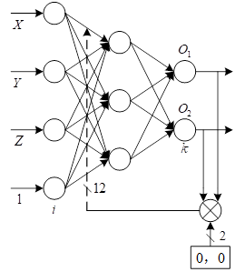
The input to the \(j\)st neuron of the hidden layer of the neural network is: \[\label{GrindEQ__13_} net_{j}^{(2)} =\mathop{\sum }\limits_{i=1}^{4} w_{ji} I_{i} ,j=1,2,3,i=1,2,3,4, \tag{13}\] where the input signals \(I_{1} ,I_{2} ,I_{3}\) and \(I_{4}\) are the coordinates of the feature points in the world coordinate system and the constant 1, respectively, and each of the weights \(w_{ji}\) of the network, respectively, corresponds to each element of the camera projection matrix.
The input to the \(k\)th neuron of the output layer is: \[\label{GrindEQ__14_} net_{k}^{(3)} =\sum _{j=1}^{3}w_{kj} O_{j}^{(2)} ,k=1,2,j=1,2,3 , \tag{14}\] where the weights \(w_{kj}\) form the matrices \(w_{kj} =\left[\begin{array}{ccc} {1} & {0} & {-u_{n} } \\ {0} & {1} & {-v_{n} } \end{array}\right]\), \(u_{i}\) & \(v_{i}\) are. The coordinates of the feature points projected to the image plane.
The excitation function \(f(x)\) of the network is a linear function, i.e: \[\label{GrindEQ__15_} f(x)=x+\theta , \tag{15}\] Where, \(\theta\) is the threshold value, which in the experiments is taken as 0 according to the pinhole model of the camera. The outputs of the neurons in the output layer and the hidden layer are \(O_{k}^{\eqref{GrindEQ__3_}} =f(net_{k}^{(3)} )\) and \(O_{j}^{\eqref{GrindEQ__2_}} =f(net_{j}^{(2)} )\), respectively.
According to the camera mathematical model, the output expectation vector of the neural network is \([0,0]^{{\rm T}}\). During the training period of the network, the performance metric of the system is obtained by the quadratic sum of the difference between the network output and the expectation value, i.e.: \[\label{GrindEQ__16_} E=\frac{1}{2} \sum _{k=1}^{2}(0-O_{k}^{(3)} )^{2} ,k=1,2 . \tag{16}\]
During neural network training, the weight matrix between the hidden layer and the output layer remains unchanged, and the weights between the input layer and the hidden layer: \[\label{GrindEQ__17_} w_{ji} (n+1)=w_{ji} (n)+\eta _{1} \delta _{j} I_{i} +\alpha _{1} (w_{ji} (n)-w_{ji} (n-1)) , \tag{17}\] where, \(\eta _{1}\) is the learning rate, \(\alpha _{1}\) is the inertia factor, and \(\delta _{j} =-\frac{\partial E}{\partial O_{j}^{\eqref{GrindEQ__2_}} } =-\sum _{k=1}^{2}O_{k}^{\eqref{GrindEQ__3_}} w_{k}\).
Adaptive genetic algorithm
Genetic algorithm is an adaptive heuristic search mechanism that includes three operations: replication, crossover and mutation [19]. In the experiment, the search space for each element in an individual is (-50000. 50000), the size of the population is \(M=80\), the number of iterations is \(T=360\), and the chromosomal individuals are obtained by a random function and take the form of a real number code. Assume that the 2 individuals are \(x_{i} =[m_{11} ,m_{12} ,\cdots ,m_{34} ]\) and \(x_{j} =[m_{11} ,m_{12} ,\cdots ,m_{34} ]\), and that there are \(x_{i} (t)=r_{1} x_{i} (t)+(1-r_{1} )x_{j} (t)\) and \(x_{j} (t)=(1-r_{1} )x_{i} (t)+r_{1} x_{j} (t)\) according to the arithmetic intersection meaning, where \(r_{1} \subset [0;1]\) is a random number. The algorithm for the non-uniform variation operation is as follows: \[\label{GrindEQ__18_} x_{in} (t)=\left\{\begin{array}{ll} {x_{in} (t-1)+(b_{i} -x_{in} (t-1)_{i} )f(t)} & {\quad if\quad 0\le \lambda _{1} <0.5}, \\ {x_{in} (t-1)-(x_{in} (t-1)-a_{i} )f(t)} & {\quad if\quad 0.5<\lambda _{1} \le 1}, \end{array}\right. \tag{18}\] where \(\lambda _{1}\) is the random number that lies between \([0,1]\). \(x_{in} (t)\) and \(x_{in} (t-1)\) are the \(n\)th variables of vector \(x_{i} (t)\), \(a_{i}\) and \(b_{i}\) are the upper and lower bounds of variable \(x_{in} (t)\), functions \(f(t)=\lambda _{2} (1-\frac{t}{T} )^{b}\), \(t\) denote the current number of generations in the iterative process, and \(T\) is the maximum number of iterations, i.e., 360. \(\lambda _{2}\) is the random number located between \([0,1]\). \(b=2\) is the shape factor.
Evolutionary speed factor
In the longitudinal direction, the direction and degree of evolution of an individual can be predicted by the evolutionary rate factor of the individual. If a chromosome is denoted as \(x_{i} (t)\) in generation \(t\) and \(x_{in} (t-1)\) in generation \((t-1)\), the distance between them is \(H_{t} (x_{i} )=\begin{array}{c} {x_{i} (t-1)-x_{i} (t)} \end{array}_{2}\). Let the interval between 2 generations be sampling unit time, the distance between 2 chromosomes \(H_{t} (x_{i} )\) can be regarded as the evolutionary speed. In this paper, let \(H_{t} (x)\) be the average distance, i.e., \(H_{t} (x)=\frac{1}{M} \mathop{\sum }\limits_{i=1}^{M} H_{t} (x_{i} )\). With reference to the normalisation process, the evolutionary speed factor can be written as: \[\label{GrindEQ__19_} e_{t} =\frac{H_{t} (x)}{\max \left(H_{1} (x),H_{2} (x),\cdots ,H_{t} (x)\right)} . \tag{19}\]
Then \(0<e_{t} \le 1\). The larger the \(e_{t}\), the faster the evolution. When \(e_{t}\) tends to 0, evolution has stalled or an optimal solution has been found.
Aggregation factor
In the horizontal direction, during the iteration process, if the diversity among individuals decreases too fast, the algorithm may not find the global optimal solution of the system. In order to describe the diversity among individuals, the concept of aggregation degree is introduced. Assuming that the centre position of all individuals in generation \(t\) is represented by vector \(x\), the sum of the distances of all individuals from \(x\) is \(d_{t} =\mathop{\sum }\limits_{i=1}^{M} ||x_{i} -x_{2} ||\), and thus the aggregation degree factor: \[\label{GrindEQ__20_} \sigma _{t} =\frac{d_{t} (x)}{\max (d_{1} (x),d_{2} (x),\cdots ,d_{t} (x))} . \tag{20}\]
It is clear that \(0<\sigma _{t} \le 1\), and the larger \(\sigma _{t}\), the better the diversity among individuals and the more dispersed they are.
Changes in the grey level of pixel points in an image produce distinct edges at the boundaries where there is a large change in grey level, which is the basis for image segmentation. However, there is a substantial difference between edges and boundaries: boundaries are the boundaries between objects in a realistic scene, because the realistic scene is three-dimensional. But the captured image is two-dimensional, and the position of the grey scale change of the pixel points in the image is called the edge. The mapping from a three-dimensional realistic environment to a two-dimensional image leads to the loss of a lot of information, whether it is the effect of noise or lighting and other factors can have an important impact on the imaging, so these reasons that do exist and can not be completely eliminated make the lack of edge extraction algorithms of the image is still a bottleneck in the digital image technology.
Laplacian operator
The Laplacian operator is a second order differential operator [3]. The matrix operator for convolution is: \[\label{GrindEQ__21_} \left[\begin{array}{ccc} {0} & {1} & {0} \\ {1} & {-4} & {1} \\ {0} & {1} & {0} \end{array}\right] . \tag{21}\]
Then the arithmetic formula is: \[\label{GrindEQ__22_} f(i,j)=f(i+1,j)+f(i-1,j)+f(i,j+1)+f(i,j-1)-4f(i,j) . \tag{22}\]
It can be seen that the second order derivatives at the boundaries are heteroscedastic, which exactly reflects the direction and strength of the image edges. This operator has no directionality and is very significant to abrupt changes in the grey scale of the image. Because the operator is a second-order operator so sensitive to image noise, so the requirements for image acquisition is higher and in the image preprocessing must first do a better smoothing.
Roberts operator
Roberts operator is two diagonally oriented differential operator which calculates the gradient of the neighbouring pixels on the diagonal [21]. The two diagonal operators are as: \[\label{GrindEQ__23_} \left[\begin{array}{cc} {0} & {1} \\ {-1} & {0} \end{array}\right]\left[\begin{array}{cc} {1} & {0} \\ {0} & {-1} \end{array}\right] . \tag{23}\]
The grey scale difference between adjacent diagonal pixel points is: \[\label{GrindEQ__24_} \Delta f_{y} =f(i-1,j)-f(i,j-1) , \tag{24}\] \[\label{GrindEQ__25_} \Delta f_{x} =f(i,j)-f(i-1,j-1) . \tag{25}\]
Then: \[\label{GrindEQ__26_} G(i,j)=\sqrt{\Delta f_{x}^{2} +\Delta f_{y}^{2} } . \tag{26}\]
Derivation of \(G(i,j)\), i.e., for the grey scale changes in 45\(\mathrm{{}^\circ}\) and 135\(\mathrm{{}^\circ}\) directions at the pixel point.Roberts operator has better directionality and high accuracy of edge position, but this operator is more sensitive to noise due to the fixed orientation and uniform treatment of the whole image.
Sobel operator
The Sobel operator is a process of comparing the magnitude of the grey scale gradient, it is not a uniform first order differentiation of the whole image, but a comparison of differentiation operations in both directions [15]. The differential convolution operator in the horizontal and vertical directions is shown in: \[\label{GrindEQ__27_} {\rm Operators\; in\; the\; y\; direction:}\left[\begin{array}{ccc} {-1} & {-2} & {-1} \\ {0} & {0} & {0} \\ {1} & {2} & {1} \end{array}\right] , \tag{27}\] \[\label{GrindEQ__28_} {\rm Operator\; in\; the\; x\; direction:}\left[\begin{array}{ccc} {-1} & {0} & {1} \\ {-2} & {0} & {2} \\ {-1} & {0} & {1} \end{array}\right] , \tag{28}\]
As can be seen from these two operators, Sobel discriminately detects the neighbours above and below and to the left and right of a pixel point, and then compares these two gradient sizes and retains the larger one, which determines that this operator has a great advantage in extracting the edge direction, but the edge position will not be guaranteed to be accurate, so there will be a case of inaccuracy of the edge position.
Canny operator
Canny operator is an optimization operator, which has the characteristics of multi-stage filtering, enhancement and detection [25].Canny operator firstly uses Gaussian filter to smooth the image to remove noise, then Canny operator uses the difference of first-order derivatives of the image to calculate the gradient magnitude and direction of the grey scale, in the whole process Canny operator also undergoes a non-maximum value suppression process, after that Canny operator is used to calculate the gradient magnitude and direction of the grey scale, and then it is used to calculate the gradient direction. In the whole process the Canny operator also undergoes a non-maximum suppression process, after which the Canny operator finally sets two thresholds to connect the edges.
The Laplacian operator is a second-order operator that is sensitive to grey scale changes and accurate in positioning, but at the same time is overly sensitive to noise, so it tends to be more affected by noise.The Roberts operator is a more diagonal differential operator, with a high degree of positional accuracy for edges, but sensitive to noise. The Sobel operator compares the vertical and horizontal gradient directions; the edge directions are accurate, but the edge locations tend to be blurred.
Variable Scale Differential Operator (VSD)
The method of image differentiation can eliminate the effect of inconsistency, through the previous analysis of various edge operators can be seen, the essence of edge extraction is a process to achieve differentiation of grey-scale map, for a variety of classical edge extraction operators, are only detecting the image changes relatively drastic region, so there is a dimension can not be more accurate extraction of image edges.
Thus, in order to extract features that are sufficiently distinguishable from slowly changing signals, a variable-scale image differentiation is proposed to solve this problem, and the operator is shown in Figure 4 (with the Sobel operator as an example).
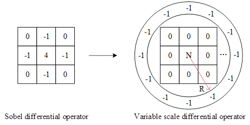
For the variable scale differential operator presented in this section, it can be seen that it is an operator that differentiates for each angle, and it is the diversity of angles that allows for a better extraction of the changes in the retarded signal.
Hough transform basic principle and implementation
Detecting a straight line using Hough transform is to transform a straight line from the original space to the parameter space [18]. The equation of a straight line is: \(y=k*x+b\), and the image space \((x,y)\) is corresponded to the slope-intercept parameter space by Hough transform. The equation of a circle is: \[\label{GrindEQ__29_} (x-a)^{2} +(y-b)^{2} =r^{2} . \tag{29}\]
Through the Hough transform, the image space \((x,y)\) corresponds to the parameter space \((a,b,r)\). In this topic, what needs to be detected is a straight line, so the main study here is to detect a straight line based on the Hough transform, and the principle is shown in Figure 5.
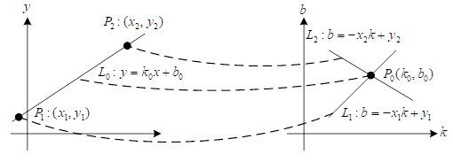
As can be seen from Figure 5, the \(x-y\) coordinate space of the original image and the parameter space \(k-b\) coordinates of the straight line have duality on the point-line, the two straight lines in the parameter space coordinates of the straight line correspond to the two points in the spatial coordinate system of the original image, and the straight line L\({}_{0}\) in the parameter space coordinates of the straight line corresponds to the point P\({}_{0}\) in the parameter space \(k-b\) coordinates.
In the \(x-y\)-coordinate, the point-sine curves are used to do the dyadic transformation due to the existence of a special case where the slope \(k\) of the 90-degree line is infinite, which affects the calculation: \[\label{GrindEQ__30_} p=x*\cos (a)+y*\sin (a) . \tag{30}\]
A point \((x,y)\) in right-angled coordinates \(x-y\) corresponds to a transformation into a sinusoidal curve in polar coordinates \(a-p\), where \(a\) is at (0-180) degrees. From the equation, it can be seen that a point \((a-p)\) in polar coordinates \(a-p\) corresponds one by one to a straight line in right-angled coordinates \(x-y\).
The polar coordinate system is micromanaged into a square grid, in the right-angled coordinate system \(x-y\) in a straight line of each point’s coordinates \((x,y)\), calculations \(p{\rm \; }={\rm \; }x*\cos (a)+{\rm \; }y*\sin (a)\), \(p\) in polar coordinates will fall in a small grid, then mark this small square number accumulator plus one, traversing the right-angled coordinate system \(x-y\) in all the points, the straight line of the point will be in the polar coordinate system will get the obvious cumulative, then counting the polar coordinates of the small squares, the accumulator of the biggest The value \((a,p)\) corresponding to the largest square corresponds to the straight line in the Cartesian coordinate system.
Hough-based target localisation
In order to avoid misjudgement due to positional errors through the algorithm firstly the part is localised in the image so that the region of interest can be determined.
For the extracted edge of the measured part, there exists a straight line at the bottom edge, which is found by Hough transform, with the slope and intercept of the straight line, the position of the part in the image can be obtained by the equation of the straight line.
In this paper, we take the bearing assembly as an example to study in depth the application of the precision component inspection model based on machine vision constructed in the previous paper in the bearing assembly.
For the same bearing standard parts in the field for 8 measurements, the size measured by the inspection model and the actual inspection size of the workpiece are compared, the component size measurement results are shown in Table 1. From the measurement data in Table 1, the maximum deviation value is 0.04mm in 8 measurements, and the maximum deviation value at each position is within the 0.05mm range required for inspection in this paper. In the eight measurements carried out in six positions did not appear to exceed the model requirements, it can be seen that the component size measurement method in this paper has excellent results.
| Number | Position 1 | Position 2 | Position 3 | Position 4 | Position 5 | Position 6 |
| 1 | 80.11 | 80.46 | 35.71 | 82.43 | 80.05 | 39.46 |
| 2 | 80.17 | 80.42 | 35.72 | 82.46 | 80.01 | 39.43 |
| 3 | 80.13 | 80.48 | 35.73 | 82.45 | 80 | 39.44 |
| 4 | 80.12 | 80.49 | 35.76 | 82.48 | 80.04 | 39.41 |
| 5 | 80.18 | 80.42 | 35.76 | 82.44 | 80.05 | 39.42 |
| 6 | 80.19 | 80.42 | 35.69 | 82.47 | 79.99 | 39.45 |
| 7 | 80.11 | 80.48 | 35.72 | 82.48 | 80.06 | 39.44 |
| 8 | 80.17 | 80.46 | 35.69 | 82.41 | 80.04 | 39.48 |
| Standard component | 80.15 | 82.46 | 35.72 | 82.44 | 80.03 | 39.45 |
In order to further quantitatively evaluate the effect of detection, standard deviation, peak signal-to-noise ratio, information entropy, and average gradient are selected as evaluation indexes in this paper. Among them, the standard deviation indicates the degree of dispersion of the grey value of the image relative to the mean value, and the more dispersed the grey level indicates the more prominent the edge of the image. The peak signal-to-noise ratio indicates the error between the corresponding pixel points, and the larger its value indicates the smaller the distortion, and the bivariate map of the edge is used as a reference in the calculation. Information entropy indicates the degree of information clutter, and larger values indicate that the image contains more information. The average gradient indicates the rate of change of the edges in the image, and a larger value indicates a clearer image.
The objective evaluation of different edge detection operator methods and the Variable Scale Differential Operator (VSD) method proposed in this paper for the edge detection of virtual model and 3D model at each angle map, five working conditions of the bearing components are selected for analysis. The results of the objective evaluation of images are shown in Table 2.
As can be seen from Table 2, for images with different acquisition modes and different targets, except for condition three, the standard deviation and peak signal-to-noise ratio of the variable scale differential operator (VSD) method proposed in this paper are better than those of the above algorithms, which indicates that the edge details detected by the variable scale differential operator (VSD) method in this paper are more accurate. The information entropy of this paper’s Variable Scale Differential Operator (VSD) method under four working conditions (except for condition three) is 0.1151, 0.0406, 0.0685, 0.1065 (all the smallest among all edge algorithms), indicating that the detected edges reduce the influence of the noise, the information is more streamlined, and the image is clearer. Edge extraction experiments on the bearing component image, although for a small number of edge mutations and irregular edges at the effect is not ideal, but for the follow-up work does not affect the majority of the edges still achieve an effective connection, and this paper’s variable scale differential method in the standard deviation, peak signal-to-noise ratio, information entropy, average gradient objective evaluation indexes are more excellent performance. In this paper, the variable scale differential operator method can effectively connect the edges of the bearing components, laying the foundation for the subsequent identification of the geometric parameters of the bearing components.
| Method | Operating condition | Evaluation index | |||
| STD | SPNR | Entropy | Mean gradient | ||
| Roberts | 1 | 51093 | 6.175 | 0.9917 | 1.1846 |
| Sobel | 80153 | 3.672 | 1.8429 | 2.6238 | |
| Laplacian | 19905 | 9.348 | 0.5429 | 0.9741 | |
| Canny | 50667 | 12.694 | 0.2048 | 1.6849 | |
| VSD | 2074 | 20.592 | 0.1151 | 2.9234 | |
| Roberts | 2 | 37468 | 7.846 | 0.7428 | 0.4685 |
| Sobel | 62488 | 5.048 | 1.3486 | 0.7816 | |
| Laplacian | 49834 | 6.297 | 1.1485 | 0.8549 | |
| Canny | 894 | 25.744 | 0.0895 | 0.1126 | |
| VSD | 85 | 35.948 | 0.0406 | 0.0689 | |
| Roberts | 3 | 40168 | 7.485 | 0.8264 | 0.5348 |
| Sobel | 70384 | 4.952 | 1.4528 | 1.2643 | |
| Laplacian | 50786 | 6.644 | 1.0535 | 1.7924 | |
| Canny | 466 | 28.45 | 0.0388 | 0.3729 | |
| VSD | 642 | 24.69 | 0.0795 | 0.8842 | |
| Roberts | 4 | 19584 | 0.523 | 1.7854 | 2.5846 |
| Sobel | 20749 | 0.384 | 2.8458 | 11.5668 | |
| Laplacian | 13665 | 2.341 | 2.6344 | 0.3874 | |
| Canny | 1285 | 20.173 | 0.0726 | 0.4682 | |
| VSD | 624 | 27.446 | 0.0685 | 0.5213 | |
| Roberts | 5 | 20485 | 0.426 | 2.0755 | 3.4825 |
| Sobel | 20146 | 0.448 | 2.8429 | 6.4872 | |
| Laplacian | 13482 | 2.647 | 2.4058 | 12.1784 | |
| Canny | 2644 | 18.488 | 0.1547 | 3.5958 | |
| VSD | 2304 | 20.648 | 0.1065 | 1.9485 | |
The geometric parameters of the bearing components are identified, and the development environment used for the experiments is as follows: the CPU is an Intel(R) Xeon(R) Platinum 8163 2.50GHz 96-core processor with 224GB of RAM, and an NVIDIA GeForce RTX 2080Ti graphics card with 12GB of video memory. The software development platform is Win10 64-bit operating system, with Pycharm as the development tool, mainly using OpenCV-Python to process edge images, using Numpy as the matrix processing of scientific computing, and Pytorch as the framework for experiments.
Referring to the products of a bearing manufacturer, the inner ring, outer ring, rolling element and cage of the bearing are taken as the research objects, and 4800 cross-section images of the bearing components are generated as the dataset by taking the original control parameters as the basis, floating within the error range of 30%, and increasing the random amount. 10% of the data, i.e., 480 edges, are randomly selected as the validation set, and the remaining 90% of the edges, i.e., 4320 edges, are used as the training set.
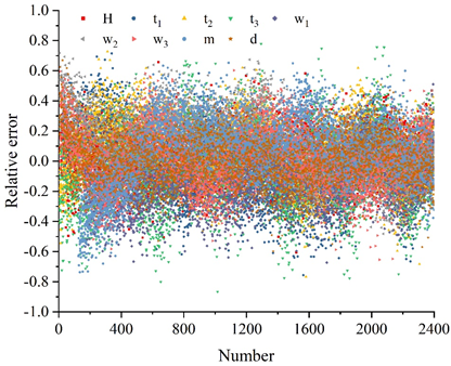
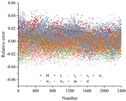
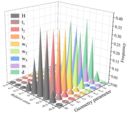
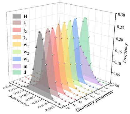
Randomly extract 2400 edge images, the detection model based on BP neural network and genetic algorithm and the fully connected neural network model of this paper are used to identify the geometric parameters of the images and calculate the relative error, the error analysis of the identification of geometric parameters of the bearing assembly cross-section is shown in Figure 6, in which Figure 6(a) is the result of the recognition of the fully connected neural network, and Figure 6(b) is the result of the recognition of this paper’s method, H, t\({}_{1}\), t\({}_{2}\), t\({}_{3}\), w\({}_{1}\), w\({}_{2}\), w\({}_{3}\), m, and d represent width, inner diameter, outer diameter, radius, contact angle, conicity, ball diameter, gap, and eccentricity, respectively. The relative error frequency of the statistical recognition results, the statistical results are shown in Figure 7.
As can be seen from Figure 6, the distribution range of geometric parameter recognition results of the fully connected neural network is larger, and almost all geometric parameter recognition results are in the interval of [-90%,80%]. The distribution range of the results of the BP neural network+genetic algorithm is smaller, and the geometric parameters basically fall within the interval of \(\mathrm{\pm}\)5%, and the recognition result error is roughly symmetrically distributed near 0. Because the BP neural network + genetic algorithm has a stronger ability to extract data features, its geometric parameter recognition results are more accurate and more symmetrically distributed.
From Figure 7, it can be seen that for the fully connected network, 68.90% of the prediction errors for gap m are within 20%, and 75.55% of the prediction errors for the other 8 key control parameters are within 20%. For BP neural network + genetic algorithm, the prediction errors of 9 key control parameters are within 5%. In terms of analysis efficiency, the performance of deep convolutional neural network in both training and prediction is much better than that of fully connected neural network, so the deep convolutional neural network is a model more in line with this application scenario, and this paper will use the deep convolutional neural network for the subsequent research.
The bearing assembly images used in the bearing assembly loosening recognition experiments were collected from the bearing manufacturers in the previous section, of which 14,000 sheets of normal assemblies and 4,000 sheets of each of the loose assemblies were used. The experiments in this section use 20,000 normal bearing assemblies and 4,000 loose bearing assemblies as the training set, and use the remaining 8,000 normal bearing assemblies and 4,000 loose bearing assemblies to match into 4,000 pairs of images of the same category and 4,000 pairs of images of different categories, in order to test the recognition performance of the precision intergroup detection model based on machine vision in this paper.
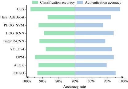
In order to verify the advantages of the method in this paper, the experiments in this section are compared with the existing methods (CIPSO, ALOK, DPM, YOLOv4, Faster R-CNN, HOG+KNN, PHOG+SVM, Harr+AdaBoost). In order to fairly compare the performance of the loss function, all methods use MSRNN network as the feature extraction network and use the same training method and training parameters. The experimental results are evaluated using two metrics: classification recognition accuracy and verification recognition accuracy, and the detailed experimental results are shown in Figure 10.
According to the experimental results, it can be seen that the classification recognition accuracy and verification recognition accuracy of the machine vision-based precision component detection model proposed in this paper are the maximum among all detection methods, and the method in this paper finally achieves the optimal recognition performance, with the classification recognition accuracy of bearing component looseness reaching 97.49% and the verification recognition accuracy reaching 98.01%, which fully proves the effectiveness of the method in this paper. It can also be seen from the experimental results that a higher recognition accuracy is achieved using verification recognition than classification recognition.
In order to verify the effectiveness of this paper’s method for detecting the angle of the bearing assembly, this paper’s method is used to detect the images of the bearing assembly at different angles. The detection results are shown in Table 3. The experimental results in Table 3 show that this paper’s model has the lowest false detection rate and leakage rate of the bearing assembly at 90\(\mathrm{{}^\circ}\), which are 0.85% and 0.28%, respectively, and the highest false detection rate and leakage rate at 270\(\mathrm{{}^\circ}\), which are 1.45% and 0.73%. In the six angles of detection, the false detection rate of this paper’s model is controlled below 1.50%, and the leakage rate is not more than 1%, which indicates that the method proposed in this paper has good detection effect in different angles.
| Angle | False detection rate/% | Undetected rate/% | Time/ms |
| 30\(\mathrm{{}^\circ}\) | 0.89 | 0.31 | 179 |
| 45\(\mathrm{{}^\circ}\) | 0.92 | 0.34 | 180 |
| 60\(\mathrm{{}^\circ}\) | 0.85 | 0.28 | 174 |
| 90\(\mathrm{{}^\circ}\) | 0.98 | 0.42 | 186 |
| 180\(\mathrm{{}^\circ}\) | 1.06 | 0.69 | 192 |
| 270\(\mathrm{{}^\circ}\) | 1.45 | 0.73 | 195 |
| Comprehensive condition | 1.03 | 0.46 | 184 |
This paper establishes a stereo vision system, uses BP neural network and heritage algorithm to calibrate the camera, and designs the detection model image processing and recognition algorithm to construct a precision component detection model based on machine vision. Taking the bearing component as an example, the component dimensions, edges, and geometric parameters are detected, and the recognition effect of components under suspicious components and different angles is tested.
In 8 measurements of the same bearing standard component, the maximum deviation value at each position is not more than 0.05 mm. The information entropy of the processing results of the edge detection method in this paper is the smallest among all edge algorithms in most cases, and the detected edge information is more streamlined and the image is clearer. The geometric parameters of the bearing components detected by the detection model in this paper basically fall within the \(\mathrm{\pm}\)5% interval, and the recognition results are highly accurate. The classification recognition accuracy of the precision component detection model based on machine vision proposed in this paper is 97.49%, and the verification recognition accuracy is 98.01%, which are the optimal recognition results among all detection methods. The comprehensive false detection rate of the component detection model in this paper is 1.09%, and the comprehensive leakage rate is 0.46%. Under the six angles of detection, the false detection rate and leakage rate of this paper’s model are kept below 1.50% and 1%, and this paper’s component detection method still has excellent detection effect under different angles.