
Portfolio optimization refers to choosing the optimal portfolio in the investment process in order to maximize the investment return or reduce the investment risk. For individual and institutional investors, portfolio optimization is an important means to achieve financial goals [7,3,2]. Stock market is a high-risk and high-return field, every day the stock market is constantly fluctuating, for investors, how to accurately predict the stock price is a very important issue. In the stock market, the trend prediction of stock price time series has been a key research direction in academia [10, 20, 18, 4], with the goal of grabbing relevant information from historical stock index prices and predicting future stock price time series data. With the development of machine learning and artificial intelligence, stock price prediction models have gradually received widespread attention [6,9,15].
Stock price prediction models can be applied in stock trading to guide investment decisions by predicting future price trends. At the same time, the stock price prediction model can also be applied in financial risk management to avoid financial risks by predicting the fluctuations of the stock market [16,12,13,5]. In addition, the stock price prediction model can also be applied in the analysis of industry and enterprise development, through the prediction of industry trends, to guide the development strategy of enterprises [19,17,22]. At the same time, the stock price prediction model can also be applied in economic forecasting, through the prediction of the stock market, to predict the trend of economic development [8,14].
In this paper, we propose to improve the basic architecture of LSTM model, on the basis of LSTM model, its encoder extracts feature information through multi-scale convolution and fuses the attention mechanism to generate a new stock price prediction model. Preprocess the stock dataset to screen the vacancy information and clarify the meaning of each code. The prediction accuracy of the improved model is evaluated using three indicators, RMSE, MAPE and MAD, as evaluation indicators. Analyze the quantitative investment model based on LSTM, and form the portfolio optimization model based on improved LSTM by combining portfolio related algorithms. Simulated trading under the consideration of risk hedging and simulated trading under the consideration of transaction cost are carried out respectively to verify the feasibility of the improved LSTM-based stock portfolio optimization model proposed in this paper.
Long Short-Term Memory Networks (LSTM) belong to a special class of Recurrent Neural Networks (RNN) and are intended to solve the problem of long term dependency that exists in recurrent neural networks [21,1].
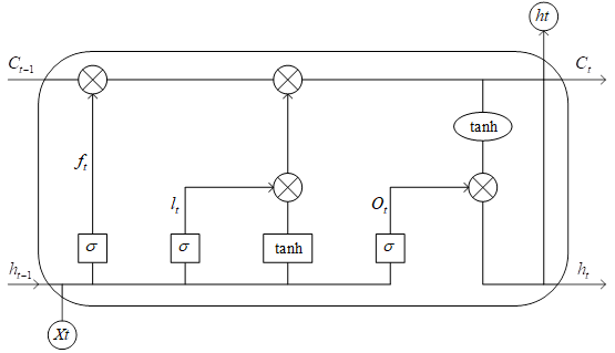
The LSTM model has four elements per cell, which are cell state \(C_{t}\), input gate \(i_{t}\), output gate \(O_{t}\) and forgetting gate \(f_{t}\). where the relevant formulas are given below: \[ f_{t} =Sigmoid(W_{f} o[h_{t-1} ,x_{t} ]+b_{f} ) ,\tag{1}\] \[i_{t} =Sigmoid(W_{i} o[h_{t-1} ,x_{t} ]+b_{i} ) ,\tag{2}\] \[C_{t} =f_{t} C_{t-1} +i_{t} \tanh (W_{c} o[h_{t-1} ,x_{t} ]+b_{c} ) ,\tag{3}\] \[O_{t} =Sigmoid(W_{o} \cdot [h_{t-1} ,x_{t} ]+b_{o} ) ,\tag{4}\] \[h_{t} =O_{t} \tanh (C_{t} ) . \tag{5}\]
In the above equation \(x\) is the input vector. \(h\) is the output vector, \(C\) is the unit state, \(t\) subscripts are the moments. Sigmoid, tanh are the activation functions, \(w\) is the weight matrix, \(b\) is the deviation matrix. The specific structure of the LSTM neuron is shown in Figure 1.
The role of the unit state is to update the information of the previous moment and integrate the information of the current moment, so as to form a memory for long-term information. The input gate determines whether the new information needs to be memorized or not, it first goes through the tanh layer to represent the information, and at the same time, it goes through the sigmoid layer to determine which information is important, and finally, it is stored with the output layer of the tanh after computation to the unit state. The result of the output gate is the current unit state weighted by the tanh. The forgetting gate determines the information that is discarded or retained in the unit state through the Sigmoid function.
In order to solve the above deficiencies, this paper splits the stock time series of multivariate features, and takes the daily closing price as the target sequence for prediction, while other variable features are categorized as exogenous sequences. The encoder extracts the features of the exogenous sequence in the time dimension through multi-scale convolution, obtains the exogenous feature information of different time spans, and generates the context vectors of the corresponding moments to be merged with the target sequence through the fusion-attention mechanism of the decoder, and outputs the prediction results through the decoder. This approach not only captures the long time dependency of the target sequence, but also considers the influence of the exogenous sequence on the target sequence at each moment. Given that this paper is forecasting the short-term price of stocks, the effect of the rise and fall of stocks on the average value of the price in the short term can be ignored without considering the short-term price mutability.
In order to integrate the effects of exogenous sequences on the target sequence at different moments, and at the same time to prevent the degradation phenomenon caused by the model being too deep, this paper proposes a new stock price prediction model MCA-LSTM.
(1) Multi-scale feature extraction: Although the exogenous sequences are not the prediction task of the model, there is no need to consider how these exogenous features interact with each other. However, each exogenous sequence variable drives the change of the target sequence, and this influence changes with the different values of the target variables at different moments. Therefore, ID convolution can be used to extract features in the time dimension from the exogenous sequence, and multiple convolution kernels of different sizes can be set up to obtain more complex multi-timescale feature information. And these different scales of information are fused as the output of the encoder, as shown in Eqs. (7) and (8): \[ f_{i,t}^{d} =Conv\left(\sum _{k=1}^{d}(W_{i,k-1} ,x_{t+k-1} ) +b_{i}^{d} \right) ,\tag{7}\] \[X_{f} =Concat(f^{d1} ,f^{d2} ,f^{d3} ,…)^{{\rm \top }} , \tag{8}\] where \(f_{i,t}^{l}\) denotes the feature value of the \(i\)rd convolutional kernel with step \(d\) of the exogenous sequence, and \(X_{f}\) denotes the feature after fusing multi-scale information.
(2) Fusion Attention Mechanism: Considering that each exogenous feature has its own semantic information, it will affect the target sequence in different dimensions at different moments. So these exogenous influences of different dimensions can be weighted and fused through the attention mechanism at each moment of the decoder. When calculating the weights, it needs to rely on the hidden state information of the decoder at the previous moment, and the fused features are called context vectors, denoted by \(c_{i}\), as shown in Eqs. (9) to (10): \[e_{t}^{i} =v_{e}^{{\rm \top }} tanh(W_{e} [h_{t-1} ;s_{t-1} ]+U_{e} X_{f}^{i} ) ,\tag{9}\] \[\alpha _{t}^{i} =\frac{\exp (e_{t}^{i} )}{\sum _{k=1}^{n}(e_{t}^{k} ) } ,\tag{10}\] \[c_{t} =\sum _{i=1}^{n}(\alpha _{t}^{i} X_{f}^{i} ) , \tag{11}\] where \(e_{i}^{i}\) denotes the score of the \(i\)nd exogenous feature to the decoder at moment \(t\), \(\alpha _{i}^{i}\) is the weight coefficient of the \(i\)th exogenous feature at moment \(t\), and \(c_{t}\) is the context vector computed with the sequence of exogenous features at moment \(t\).
The \(\tilde{y}_{i}\) obtained by combining the context vector \(c_{i}\) and the input \(y_{i}\) of the decoder can be used to update the hidden state of the decoder at the moment \(t\) as shown in equation (12). Namely: \[\label{GrindEQ__12_} \tilde{y}_{t} =\tilde{W}^{{\rm \top }} \left[\begin{array}{c} {y_{t} ;c_{t} } \end{array}\right]+\tilde{b} . \tag{12}\]
In this paper, we mainly collect the data of constituent stocks in CSI 300 index to construct the stock dataset, and the data are obtained from Yahoo Finance platform [11].
In the process of dataset construction, the individual stock stock samples that are representative of the market are selected from the 300 stock stock samples. The data are downloaded from the official channels of Yahoo Finance and saved in CSV format in My SQL database for unified management and maintenance.
The trading data of 20 CSI 300 constituent stocks from January 16, 2012 to December 31, 2022 were obtained through the public data interface provided by Yahoo Finance as the most important data collection object. Through the data acquisition results, the mismatched data volume is eliminated. Due to the lack of the original data, it is necessary to do appropriate preprocessing of the acquired stock price data before it can be stored in the My SQL database and used as the data base for the empirical study.
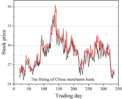
After data preprocessing, taking the individual stock data of China Merchants Bank (stock code 600036) as an example, the results of data set processing are shown in Table 1. In the table, code is the stock code, date is the date, and YYYYMMDD is the standard format, such as 20120116. Open is the opening price and CLOSE is the closing price. High is the highest price, low is the lowest price, and volume is the turnover. On January 16, 2012, the highest price of China Merchants Bank (stock code 600036) was 18.27.
| Code | Date | Open | Close | High | Low | Volume |
| 600036 | 20120116 | 17.63 | 17.33 | 18.27 | 17.02 | 756923.21 |
| 600036 | 20120117 | 18.43 | 18.15 | 18.45 | 17.89 | 905361.57 |
| 600036 | 20120118 | 19.04 | 18.46 | 19.15 | 18.55 | 792213.44 |
| 600036 | 20120119 | 18.66 | 17.74 | 18.71 | 17.74 | 102469.06 |
| 600036 | 20120120 | 16.75 | 16.85 | 16.89 | 16.25 | 836045.01 |
| 600036 | 20120121 | Weekend rest | Weekend rest | Weekend rest | Weekend rest | Weekend rest |
| 600036 | 20120122 | Weekend rest | Weekend rest | Weekend rest | Weekend rest | Weekend rest |
| 600036 | 20120123 | 16.75 | 16.25 | 16.81 | 16.21 | 146926.37 |
| 600036 | 20120124 | 18.69 | 17.64 | 18.74 | 17.62 | 113625.08 |
After preprocessing, the stock price data ensures that the length of time of each constituent stock is consistent and the time order of the data is strictly guaranteed. The time series data in this project is in the frequency of days, which contains more than 620,000 stock price data, and the subsequent experimental research will be carried out on the basis of this dataset.
| Configuration item | Configuration |
| Programming language | Python |
| Third-party libraries used | pandas, numpy, matplotlib.pyplot, tensorflow, scipy.spatial.distance |
| Neural cryptography | 12 |
| Neural network input data dimension | 8 |
| Neural network output layer number | 2 |
| Batch _size | 3 |
| Time_step | 9 |
| Learn rate | 0.0003 |
The corresponding experimental results for all 12 stocks are then shown in Table 3.
| Experimental sample | RMSE | MAPE | MAD |
| Guizhou maotai 600519 | 28.6539 | 6.122 | 26.078 |
| China ping an 601318 | 18.9664 | 17.003 | 2.99 |
| Grain liquid 000858 | 1.3651 | 1.891 | 0.912 |
| China merchants bank 600036 | 0.5399 | 1.424 | 0.431 |
| Hengrui 600276 | 1.1243 | 1.739 | 0.897 |
| Citic securities 600030 | 0.3651 | 0.634 | 0.102 |
| Gree electric appliance 000651 | 4.3005 | 6.528 | 3.365 |
| Yili shares 600887 | 0.5872 | 1.469 | 0.421 |
| China free 601888 | 0.4175 | 1.034 | 0.365 |
| Societe generale 601166 | 0.2693 | 0.728 | 0.142 |
| Vanke A 000002 | 7.1694 | 16.162 | 5.396 |
| ICBC 601398 | 0.0981 | 1.408 | 0.072 |
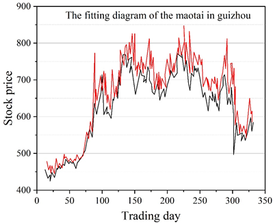
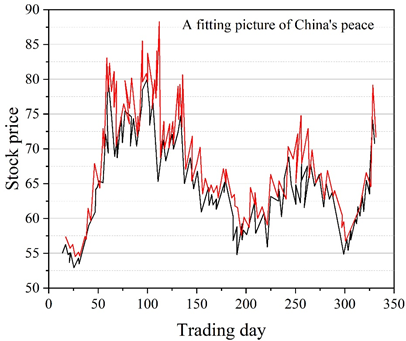
The improved LSTM model has smaller prediction errors on most stock samples. However, there are still some samples with large errors between the predicted and actual values, such as Guizhou Maotai (600519) and Ping An of China (601318). The RMSE values of Guizhou Maotai and Ping An of China reach 28.6539 and 18.9664, respectively.
By analyzing the data sample can be obtained, the above stocks data base is larger compared to other stocks, their closing price data is generally in the thousands. While most of the other stocks sample closing price is a few dollars to a few hundred dollars ranging, the above two stocks and other stocks with a large difference in value. So the fluctuation range of the predicted value is also much higher than most other stock samples.
Through the analysis of the above experimental results, it can be concluded that the performance of the short-term and long-term memory network model in the problem of stock closing price prediction has achieved the expected results, but in some sample data need to make the corresponding normalization of the data and the adjustment of the model parameters so that the model can get a more ideal effect.
The model aims to achieve the following objectives:
On the one hand, the model predicts the return of the stock and visualizes the potential trend of the stock, so as to provide investors with a reference for decision-making.
On the other hand, through the risk indicators of the model, the risk level of the transaction is assessed so that investors can better manage the risk and maximize the return.
The overall framework of the model is shown in Figure 3. In this framework, the stock data are first predicted using the LSTM model to obtain the predicted returns, and this step takes advantage of the LSTM model’s strengths in handling time series data, which can capture the long-term dependencies in the data to more accurately predict the future returns. Next, through risk assessment of the model output returns, corresponding risk indicators can be obtained, which can reflect the risk level of the trading strategy, helping investors to consider the risk factors when making decisions and make corresponding adjustments according to their own risk tolerance. Finally, based on the results of the model prediction and risk assessment, investors can formulate the corresponding trading strategy and conduct live trading. In this way, investors can trade according to the guidance of the model in a real-time market environment in order to realize the value-added of their investment portfolios.
The improved LSTM-based quantitative stock investment model plays an important role in the establishment of the LSTM-based quantitative stock investment methodology, the automated trading function of the live market, and helps investors to make informed investment decisions and maximize their returns during the investment process by providing yield prediction and risk assessment.

Using \(E\) to denote the expected return and \(\delta ^{2}\) to denote the variance, the mean-variance model expression is shown in Eq. (13). Namely: \[\label{GrindEQ__13_} \left\{\begin{array}{l} {min\delta ^{2} (r_{p} )=\Sigma \Sigma w_{i} w_{j} cov(r_{i} ,r_{j} )}, \\ {E(r_{p} )=\Sigma w_{i} r_{i} }, \end{array}\right. \tag{13}\] where \(r_{p}\) is the portfolio return. \(w_{i}\) is the weight of asset \(i\) in the portfolio, and \(r_{i}\) is the return on asset \(i\). \(cov(r_{i} ,r_{j} )\) is the covariance between asset \(i\) and asset \(j\).
The model can be solved by the Lagrange method, which solves for the weights of the assets that minimize the risk of the portfolio when the expected rate of return is determined.
Economically speaking, an investor can minimize the overall investment risk by determining the expected rate of return before investing, and then obtaining the weights of each asset. Each different expected return corresponds to a different portfolio weighting solution, which together form the efficient portfolio, i.e., the portfolio with the lowest variance. The curve formed between the expected return of the efficient portfolio and the corresponding minimum variance is called the efficient frontier of the portfolio. Investors will choose the portfolio solution with the highest utility on the efficient portfolio frontier based on different return expectations and risk-taking levels.
(1) Capital asset pricing model: Based on the assumptions in modern portfolio theory, other assumptions in CAPM show a complete capital market, i.e., the absence of any frictions that discourage investment, including the ability of investors to borrow or lend any funds without restriction at the level of the risk-free rate of interest, the absence of fees and taxes for trading securities, and the possibility of unlimited splitting of security shares.
The CAPM expression for a single stock or portfolio is shown in Eq. (14). Namely: \[\label{GrindEQ__14_} \bar{r}_{t} =r_{f} +\beta _{i} (\bar{r}_{m} -r_{f} ) , \tag{14}\] where \(\bar{r}_{i}\) is the expected rate of return on a single stock \(i\) or portfolio \(i\). \(r_{f}\) is the risk-free rate of return, \(\beta _{i}\) is the \(\beta\) coefficient of the asset \(i\) or portfolio \(i\). \(\bar{r}_{m}\) is the expected return of the market portfolio.
The CAPM gives a simple conclusion that there is only one factor that will lead to a higher return on investment, and that is investing in risky stocks.
(2) Sparse and stable portfolio selection: For a standard portfolio selection problem with \(N\) risky asset, at moment \(t\), the excess return \(R_{t}\) obeys a multivariate normal distribution with mean \(\mu\) and variance-covariance matrix 2, where \(\mu\) is a \(N\times 1\)-dimensional column vector and \(\Sigma\) is an \(N\times N\)-dimensional matrix. At moment \(t\), the investor needs to determine the portfolio weights \(w\) to maximize the mean-variance objective function as shown in Eq. (15). Namely: \[\label{GrindEQ__15_} U(w)=w^{T} \mu -\frac{\gamma }{2} w^{T} \Sigma w , \tag{15}\] where \(U\) is the utility obtained by the investor. \(\gamma\) is the investor risk aversion coefficient. The optimal portfolio weight is \(w=\gamma ^{-1} \Sigma ^{-1} \mu\).
And for the multiple linear regression with \(N\) independent variables and \(N\) observations \(y=Xw+e\), \(e\) is the random error term that makes: \[\label{GrindEQ__16_} \left\{\begin{array}{l} {X=\sqrt{\gamma } \Sigma ^{-\frac{1}{2} } } ,\\ {y=\frac{1}{\sqrt{\gamma } } \Sigma ^{-\frac{1}{2} } \mu }. \end{array}\right. \tag{16}\]
Then the least squares estimator of the multivariate linear regression, \(\hat{w}_{oLS} =(X^{T} X)^{-1} (X^{T} y)\), equals the optimal portfolio weights, \(\hat{w}=\gamma ^{-1} \Sigma ^{-1} \mu\). In other words, the least squares estimator solves the portfolio selection problem.
Since investors do not know the real \(\mu\) and \(\Sigma\), among the estimators based on historical data, the great likelihood estimators \(\hat{\mu }\) and \(\hat{\Sigma }\) are widely used, and then the optimal portfolios are found by Eq. (17). Namely: \[\label{GrindEQ__17_} U(w)=w^{T} \hat{\mu }-\frac{\gamma }{2} w^{T} \hat{\Sigma }w . \tag{17}\]
There are three sources of estimation error in Eq. Estimated mean \(\hat{\mu }\), estimated covariance matrix \(\hat{\Sigma }\), and inverse matrix of estimated covariance matrix.
When the number of assets is large, a sparse portfolio needs to be constructed. First, a sparse portfolio reduces transaction and management costs. Second, by setting the weights of smaller portfolios to zero, the estimated portfolio weights are no longer unbiased, but their variance and mean-square prediction errors can be reduced. Sparse portfolio weights can be obtained by imposing Lasso constraints on the portfolio weights. The portfolio weights are estimated through Eq. (18). Namely: \[\label{GrindEQ__18_} \hat{w}_{L1} =argmax\left\{w^{T} \hat{\mu }-\frac{\gamma }{2} w^{T} \hat{\Sigma }w\right\} s.t.||w||_{1} <s_{1} , \tag{18}\] where \(s_{1}\) is a constant greater than zero.
When \(s_{1} >0\), the portfolio weights \(\hat{w}_{L1} =(\hat{w}_{L1,1} ,…,\hat{w}_{L1,N} )^{T}\) shrink toward zero. If the OLS estimates are small enough in absolute value, the penalized least squares \(\hat{w}_{L1,j}\) is exactly zero.
In mean-variance efficient portfolios, extreme weights usually occur and portfolio weights can change significantly when new return information is used and when a set of assets is not available for trading. This is caused by large estimation errors in the inverse matrices of \(\Sigma\) and \(\hat{\Sigma }\). When the returns of the two assets are highly correlated, the inverse matrix of \(\hat{\Sigma }\) becomes highly unstable and causes the weights of the two assets to fluctuate substantially over time. Therefore, imposing stability constraints is expected to reduce the estimation risk due to parameter uncertainty and multicollinearity. Replace \(\hat{\Sigma }\) with \(\hat{\Sigma }_{s} =v\hat{\Sigma }+(1-v)\hat{\Sigma }_{g}\), where \(\hat{\Sigma }_{g}\) is a contraction target with low variance and \(v\) is the contraction intensity. This is equivalent to imposing a constraint on the sum of squares of the portfolio weights.
The portfolio weights can be estimated by Eq. (19). Namely: \[\label{GrindEQ__19_} \hat{w}_{L1L2} =argmax \left\{w^{T} \hat{\mu }-\frac{\gamma }{2} w^{T} \hat{\Sigma }w\right\} s.t.||w||_{1} <s_{1} ,||w||_{2}^{2} <s_{2} . \tag{19}\]
When \(s_{1} >0\) and \(s_{2} >0\), the portfolio weights are first scaled and then contracted towards zero, thus improving the sparsity and stability of the constructed portfolio.
In this study, we optimize the LSTM to predict the future returns of stocks to achieve the goal of obtaining the subjective viewpoint parameters of the BL model, and input them into the BL model to obtain the allocation weights of the stock portfolio. And the assets are allocated in accordance with the model output, constituting the MCA-LSTM-BL stock portfolio model.
(2) Portfolio optimization model based on improved LSTM network return prediction: Based on the framework of the mean semi-absolute deviation (MSAD) portfolio optimization model, a new portfolio optimization model based on return prediction is established. That is, the portfolio optimization model based on improved LSTM network return prediction (MCA-LSTM +MSAD).
In order to test the performance of the MCA-LSTM stock portfolio model in terms of arbitrage and generalization, this section applies the analysis of the MCA-LSTM-BL model in terms of data sources, indicator factor selection and parameter setting, model evaluation indexes, and comparative analysis between the model and the data to further demonstrate the practical value of the model.
The research data are still selected from the same stocks as in the previous section, the constituent stocks in the January 2022 stock pool of CSI 300 index. The daily frequency data is from January 16, 2012 to December 31, 2022 by applying the analysis to the stocks.
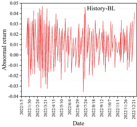
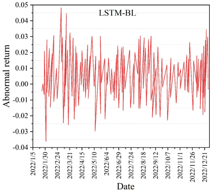
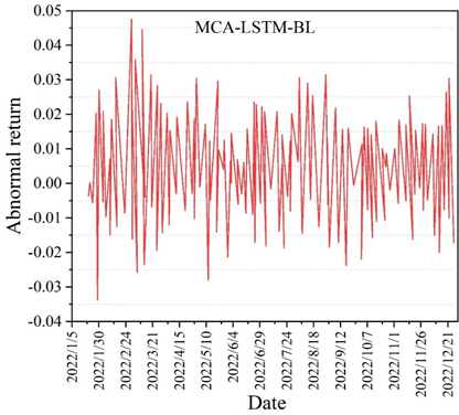
The two models, MCA-LSTM-BL and LSTM-BL, mainly use the returns predicted by the MCA-LSTM model and the LSTM model as the viewpoint returns input into the BL model. Since the LSTM model belongs to the time-series model, which is more sensitive to recent data and is not suitable for predicting too long a time period in the future, this paper adopts a rolling training approach, where every 50 days, the model is trained using data from the past 100 days, and the results of the yields for the day’s backward 50 days are predicted, and so on, until the end of the training set.
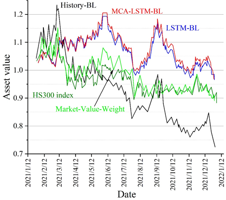
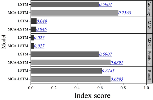
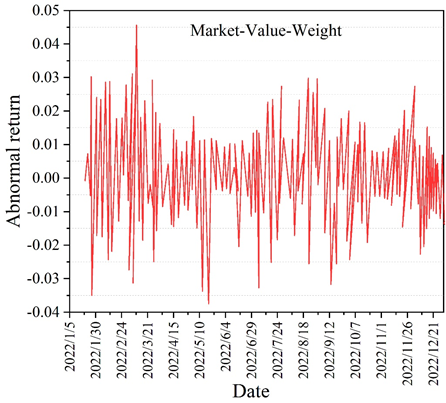
The errors of the two prediction methods in the comparison of the datasets are slightly higher compared to the previous ones, but they also reflect a good performance within the acceptable range. The five comprehensive measures of the model’s predictive ability in the table reflect that MCA-LSTM outperforms LSTM, with the Accuracy of MCA-LSTM being 0.7568. This indicates that the MCA-LSTM model has high accuracy and generalization ability in yield prediction. The differences between the different model portfolio returns and the market stock index returns are compared under the new data set. The different model abnormal return curves are shown in Figure 6. The difference between different portfolios and the HS300 index market is reflected by the different modeled abnormal return curve plots in the figure. Also in the comparison, it can be concluded that the MCA-LSTM-BL model has the smallest fluctuation and the smoothest amplitude of the portfolio abnormal return (which is equivalent to the excess return here), which still shows a good stability, and similarly in contrast to the market capitalization weight methodology, although there are sporadic and more prominent highs in the test set, there is a negative return in high frequency, and there is less fluctuation near the zero, which shows that the portfolio represented by its model cannot bring stable excess returns and the investment effect is not satisfactory. Through the experimental comparison, it can be concluded that the MCA-LSTM-BL stock portfolio model has a good return.
Among all DNNs, Long Short-Term Memory (LSTM) networks and Convolutional Neural Networks (CNNs) are the most commonly used models for stock price prediction. Therefore, the purpose of this section is to further improve the out-of-sample performance of return prediction-based portfolio optimization models by using LSTM networks and CNNs.
Based on the framework of the mean semi-absolute deviation (MSAD) portfolio optimization model, a new return prediction-based portfolio optimization model is developed. In order to illustrate the merits of these models, three equally weighted portfolio models are selected in this section for comparison, who select their stocks using improved LSTM, LSTM network and CNN, respectively. And two portfolio models based on Support Vector Regression (SVR) return prediction are used as benchmarks, and they use SVR instead of DNNs for return prediction.
It is well known that trading costs can have a significant impact on the returns of trading strategies. And a high turnover rate can lead to high trading costs. Therefore, it is meaningful to test the actual performance of the portfolio optimization model based on return prediction after deducting the trading costs. For simplicity, this section only considers a 0.06% per unit turnover rate to study the performance of different models.
This section applies \(R_{p} =0.03\) to discuss the performance of different portfolio optimization models based on return forecasting. The performance of different models considering transaction costs is shown in Table 4. ER, SD, IR, TR, and MD are denoted as excess return, standard deviation, informatization rate, total return, and maximum retracement, respectively. The improved LSTM algorithm with mean semi-absolute deviation (MSAD) portfolio optimization model proposed in this paper is able to achieve 56.98% excess return.
| Model | ER | SD | IR | TR | MD |
| MCA-LSTM+ MSAD | 0.5698 | 0.5962 | 0.9175 | 1.9637 | 0.7542 |
| LSTM+ MSAD | 0.1025 | 0.2028 | 0.4938 | 1.4604 | 0.4138 |
| CNN+ MSAD | -0.0517 | 0.0905 | -0.4614 | 0.2976 | 0.5446 |
| SVR+ MSAD | -0.1493 | 0.1834 | 0.8993 | -0.0428 | 0.5299 |
| SVR+MV | -0.2115 | 0.4617 | 0.4352 | -0.2013 | 0.5867 |
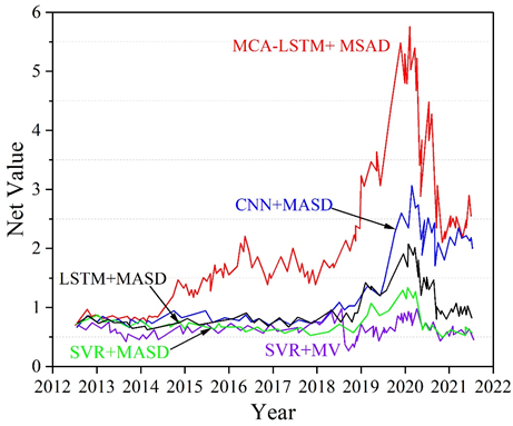
The net values of the different models considering transaction costs are shown in Figure 7, which directly shows the performance of the different models on the out-of-sample test set. The MCA-LSTM+MASD model is able to maintain the maximum value consistently over the stock trading day period 2012-2022 and with an \(R_{p}\) value of 0.03. This paper concludes that MCA-LSTM+MASD is a promising model for portfolio optimization in real investment.
In this paper, a new stock price prediction model MCA-LSTM is proposed by improving the long and short-term memory network algorithm, adding multi-scale feature extraction and attention mechanism, screening and processing the stock dataset, and utilizing the new prediction model to make the time series prediction of stock price. Considering the stock return prediction to form a stock portfolio, the investment efficiency optimization analysis is performed with the help of evaluation indexes.
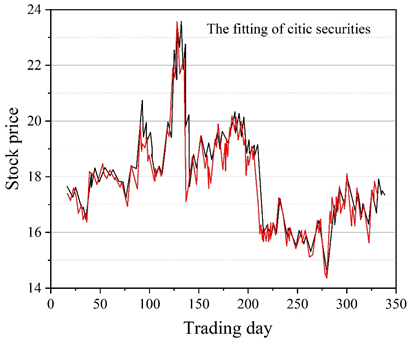
The improved LSTM stock price prediction model has smaller prediction errors for the four samples of Guizhou Moutai, Ping An of China, CITIC Securities, and China Merchants Bank, which are in line with the demand for predicting price changes in the stock market.
Combining the quantitative investment framework of LSTM and substituting it into the improved LSTM stock price prediction model, it constitutes a portfolio optimization model based on the improved LSTM. In the simulated trading considering risk hedging, the MCA-LSTM-BL model has the highest portfolio asset value and the best return generated by the portfolio, which better validates the stability of the model. The composite measure of predictive ability index of each prediction model reflects that MCA-LSTM outperforms LSTM in all cases, with the Accuracy of MCA-LSTM being 0.7568. This indicates that the MCA-LSTM model has a high accuracy and generalization ability in yield prediction.
Also under the condition of considering the transaction cost, the portfolio strategy based on the improved LSTM model proposed in this paper can achieve the maximum excess return, which verifies that the MCA-LSTM portfolio model proposed in this paper can be established out-of-sample. Thus, this paper concludes that the MCA-LSTM portfolio model is capable of optimizing portfolio returns in real investment.