
With the popularization of electric vehicles and the development of power distribution network, charging pile as an important facility for electric vehicle charging has gradually received attention. Charging piles can not only realize the rapid charging of electric vehicles, but also realize the efficient use of energy through the coordinated operation with the distribution grid. In the face of large-scale charging piles, its operation mode includes charging pile layout, charging strategy, and main grid interaction [15, 25]. Under the background of smart grid, the charging pile is interconnected with the grid through information and communication technology to realize the intelligent control of the charging pile and the intelligent scheduling of the grid. This interaction can make the charging of electric vehicles more intelligent and efficient, improve energy utilization efficiency, reduce energy waste, and promote the use of clean energy and the development of smart grid [19, 17, 18].
As a small power generation and distribution system composed of multiple distributed energy resources, microgrids can be operated independently or grid-connected, with a certain degree of autonomy and flexibility [4]. Grid-connected operation means that the microgrid is connected to the main grid, and energy sharing and complementarity is realized by communicating with the main grid [12]. And the optimization of microgrids aims to improve energy efficiency, reduce operating costs, energy storage management and power supply reliability. Among them, ensuring the reliability of power supply is the primary task of microgrid operation optimization, which can improve the reliability of power supply by connecting with the main grid to obtain emergency backup energy to cope with possible energy shortage [2, 20]. The interconnection and cooperative operation between microgrids and smart grids are realized through information and communication technology and intelligent control technology to jointly improve the security, stability and economy of the power system [13].
Existing large-scale charging pile designs do not pay attention to the charging station load problem, which can easily lead to overloading or damage of the distribution transformer. For this reason, a real-time monitoring and control system for distribution transformer load is designed for literature [10], which is operated under the proposed charging pile coordination strategy to optimize the output power of the charging pile and prevent the distribution transformer from overloading. Literature [26] constructs a vehicle-pile-network interconnection framework based on the interconnection between electric vehicles, charging piles, and power grids, while literature [24] directly develops an optimization technique for the interaction between electric vehicle charging piles and power grids, which achieves charging pile load power smoothing, and reduces the pressure caused by charging pile loads on distribution transformers. In the case of large-scale charging, the charging pile distribution grid is prone to node undervoltage conditions, and literature [21] designed a hybrid charging management system to solve the problem. In addition to the optimization of the technical level, large-scale charging piles must need to consider the cost and revenue issues, literature [23] obtained the optimal distribution scheme of large-scale charging piles through the Erlang-Loss system under the consideration of multiple constraints, such as charging demand, range, human activities, and the charging process, which alleviated the supply-demand relationship between the charging demand and the tension of charging resources. The planning of charging piles should not only consider issues such as distance and energy consumption, but also cost and profitability. Literature [8] has studied the multi-objective charging path planning for electric vehicles under multiple pricing models, while optimizing the best pricing model based on benefit maximization and profit balance. And literature [9] uses model-free deep reinforcement learning for decentralization to solve the optimal solution for real-time scheduling of large-scale EV charging, which is also beneficial to the stochastic charging problem on the basis of cost minimization.
Currently, the commonly used techniques and algorithms for microgrid operation optimization are mixed integer planning techniques, multi-agent’s techniques, meta-heuristic algorithms, genetic algorithms, and simulated annealing algorithms [7], of which the first three are widely used due to the simplicity and high efficiency of optimization procedures or excellent optimization results for energy management [16]. The uncertainty of renewable energy sources does pose a challenge to the stage of microgrid operation planning, for this reason, literature [1] constructed a multi-stage stochastic planning model for microgrid operation based on variable renewable energy sources, energy storage systems, and thermal generating units, and the fluctuation of energy sources needs to be emphasized for both long term and short term planning, especially when the uncertainty is high and the dispatchability is limited. The high operating cost has been one of the problems in microgrids, for this reason, literature [5] developed a hybrid microgrid operation optimization method considering the weather factor, where long term planning is more favorable under cost minimization, but this period does not have continuity. Literature [11] optimized the fuel cost of dispatchable distributed generation in microgrid operation through four techniques: lambda iteration, lambda logic, direct search method, and particle swarm optimization. However, as far as the current study is concerned, there is a lack of accurate scheduling and demand forecasting in energy management for microgrid operation, and the impact of distributed energy fluctuations has not been fully addressed, and there is a lack of intelligent scheduling at the market application level.
In this paper, parameters related to the optimal scheduling of EVs are generated with reference to the types of EVs and their charging methods and driving characteristics, and the information is entered into the network. Subsequently, Monte Carlo simulation is used as a charging demand simulation method based on charging probability modeling. The Monte Carlo method is used to analyze and process the data sampling of the grid entry parameters to obtain the probability density function distribution. Based on the distribution parameters, the EV sequential charging model is established. Considering the user’s response, the clean energy scheduling strategy for grid-connected operation of microgrid is proposed. Based on the EVs charging model, the classification of scheduling control strategies is realized. For the centrally controlled microgrid, the construction of the microgrid operation optimization model is completed by combining the load changes generated by different response behaviors of users, and the relevant constraints are proposed. Through the adaptive particle swarm optimization algorithm, the solution of the model is realized. Simulation experiments are designed to verify the feasibility of the model, and at the same time, different conditions are set according to different user response states to study the output of controllable generation units.
Electric vehicles use batteries as the main power source and are driven wholly or partially by electric motors [3]. According to the current technological level and vehicle driving principle, electric vehicles can be divided into three categories: pure electric vehicles (PEVs), plug-in hybrid electric vehicles (PHEVs), and fuel cell electric vehicles (FCEVs). Among them, pure electric vehicles are powered entirely by secondary batteries, such as nickel-metal hydride batteries, nickel-cadmium batteries and lithium-ion batteries, etc. Battery power is supplemented by the charging system, which can truly realize “zero emission”, and is the future development direction of the automotive industry.
According to the research, the average daily mileage of the bus is about 150-200km, in order to meet the normal operational needs of the bus, it needs to be charged 2 times a day, daytime buses in the operating hours 06:00-24:00, using fast charging, according to the calculation of a round trip of 4h, the charging load in the time period of 10:00-20:00 to meet the uniform distribution, the beginning of charging \(SOC\) to meet the normal distribution. \(N\left(0.5,0.1^{2} \right)\), night buses in non-operating hours 0:00-06:00, the use of conventional charging, charging load in the period to meet the uniform distribution, and to meet the start of operation when the battery SOC is 0.95, the start of charging SOC also meet the normal distribution \(N\left(0.5,0.1^{2} \right)\).
The average daily mileage of the cab is about 350-500km, and the cab needs to be charged twice a day to meet the operational demand. In order to avoid charging congestion during the peak period of handover, it is assumed that the charging load of cabs meets the uniform distribution throughout the day, i.e., the starting charging time meets the uniform distribution throughout the day, and the starting charging SOC meets the normal distribution \(N\left(0.3,0.1^{2} \right)\), and fast charging mode is adopted.
When the official car is not performing tasks, it can be charged, and in most cases, the official car has enough charging time, and it can be charged once a day to meet the demand. Assuming that the official car is charged after work, the battery SOC is 0.95 before the next day’s work, i.e., the charging period is 18:00-07:00, the charging load meets the uniform distribution during the period, and the starting charging SOC meets the normal distribution \(N\left(0.4,0.1^{2} \right)\), and conventional charging mode is adopted.
In general, the daily mileage of private cars depends on the user’s driving habits, assuming that the charging behavior is also only affected by the user’s driving habits, according to the U.S. Department of Transportation NHTS2009 research results, the use of great likelihood to estimate the user’s daily mileage to satisfy the lognormal distribution, and its probability density is: \[\label{GrindEQ__1_} f_{D} (d)=\frac{1}{d\sigma _{D} \sqrt{2\pi } } \exp \left(-\frac{\left(\ln d-\mu _{D} \right)^{2} }{2\sigma _{D}^{2} } \right). \tag{1}\]
EV has many parameters, and the parameters of interest in EV optimal scheduling are battery nameplate parameters such as battery capacity, charging efficiency, etc., grid entry parameters, and operational parameters such as state of charge SOC, state of charge, charging power, and grid-connected state.
EV charging optimization scheduling algorithms are divided into two parts: charging demand simulation and ordered scheduling algorithms [6]. The commonly used charging demand simulation method based on charging probability modeling represented by Monte Carlo simulation is described below.
Currently charging demand simulation is mainly divided into the following two categories according to the need to generate the parameters for network entry.
The first entry parameter is based on the NHTS to generate the entry time \(t_{s}\), exit time \(t_{e}\), and mileage \(d\). Assuming that the private EV user connects to the charging device to charge at home at the end of the trip until he leaves home on the next day, the EV entry time and exit time correspond to the time of connecting to the charging post and leaving the charging post, respectively. According to \(t_{s}\) and \(t_{e}\), we can calculate the length of stay, and according to \(d\), we can calculate the charging demand and charging time. \(t_{s}\), \(t_{e}\), \(d\) obey the following segmented normal distribution \(f_{s} (x)\), segmented normal distribution \(f_{e} (x)\), lognormal distribution \(f_{d} (x)\), respectively: \[\label{GrindEQ__2_} f_{s} (x)=\left\{\begin{array}{c} {\frac{1}{\sigma _{s} \sqrt{2\pi } } \exp \left[-\frac{\left(x-\mu _{s} \right)^{2} }{2\sigma _{s}^{2} } \right],\qquad ~~~~\mu -12<x\le 24}, \\[4mm] {\frac{1}{\sigma _{s} \sqrt{2\pi } } \exp \left[-\frac{\left(x+24-\mu _{s} \right)^{2} }{2\sigma _{s}^{2} } \right],\qquad 0<x\le \mu -12}, \end{array}\right. \tag{2}\] \[\label{GrindEQ__3_} f_{c} (x)=\left\{\begin{array}{c} {\frac{1}{\sigma _{e} \sqrt{2\pi } } \exp \left[-\frac{\left(x-24-\mu _{c} \right)^{2} }{2\sigma _{c}^{2} } \right],\qquad~~~ \mu _{e} +12<x\le 24}, \\[4mm] {\frac{1}{\sigma _{e} \sqrt{2\pi } } \exp \left[-\frac{\left(x-\mu _{c} \right)^{2} }{2\sigma _{c}^{2} } \right],\qquad ~~~~~0<x\le \mu _{e} +12}, \end{array}\right. \tag{3}\] \[\label{GrindEQ__4_} f_{d} (x)=\frac{1}{x\sigma \sqrt{2\pi } } \exp \left[-\frac{(\ln x-\mu )^{2} }{2\sigma ^{2} } \right], \tag{4}\] where \(\mu _{s} =17.5\), \(\sigma _{s} =3.5\), \(\mu _{e} =9.24\), \(\sigma _{e} =3.16\), \(\mu =3.7\), \(\sigma =0.92\).
Then the charging duration \(t_{ch}\) is calculated as follows: \[\label{GrindEQ__5_} t_{ch} =\frac{\left(SOC_{end} -SOC_{ini} \right)C}{P_{c} \eta _{c} } =\frac{dE_{100} }{100P_{c} \eta _{c} } , \tag{5}\] where, \(E_{100}\) is the power consumption for 100km traveling. \(C\) is the EV battery capacity. \(SOC_{ini}\) is the in-grid state of charge, \(SOC_{end}\) is the desired off-grid state of charge. \(P_{c}\) is the constant charging power. \(\eta _{c}\) is the EV charging efficiency.
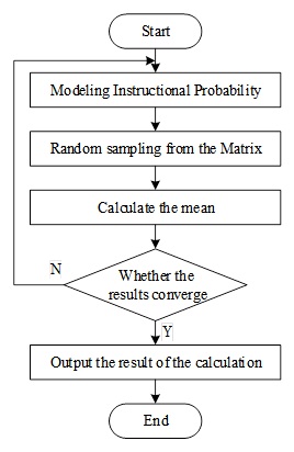
Monte Carlo method is also known as statistical experiment method and random sampling method [22]. The Monte Carlo method can be used to analyze the data sampling of the grid entry parameters very well. The Monte Carlo simulation flowchart is shown in Figure 1 as shown. Taking 1000 EVs as the number of simulated EVs, the Monte Carlo generated \(t_{s}\), \(t_{e}\), \(d\) statistics and probability density of 1000 EVs are obtained. Monte Carlo simulation generates statistics of the frequency distribution histogram envelope and probability density function is extremely similar, when the number of simulated EVs is large enough or the number of repetitions is sufficiently large, the closer the two should be, the distribution of statistical data obeys the distribution of the probability density function.
The second entry parameter includes entry time \(t_{{\rm s}}\), exit time \(t_{{\rm e}}\), entry charge state \(SOC_{ini}\), and expected exit charge state \(SOC_{end}\). Since the second parameter contains more and more comprehensive parameters, which is favorable for the preparation of the orderly charging and discharging scheduling algorithm, the second entry parameter is adopted in the following section without any explanation. It is assumed that the EV entry parameters of community MG1 and park MG2 follow the distribution, and Table \(N(x,y)\) indicates normal distribution and \(U(x,y)\) indicates mean value distribution. In the paper, the scheduling interval is 1h, and the rounding operation must be performed on \(t_{s}\) and \(t_{e}\): \[\label{GrindEQ__6_} t_{s} =\left\lceil t_{s} \right\rceil ,t_{c} =\left\lceil t_{c} \right\rceil , \tag{6}\] where \(\left\lceil\;\; \right\rceil\) denotes upward rounding.
Firstly, according to the distribution parameters, the EV cluster entry information of community MG1 is generated based on Monte Carlo simulation, which includes entry time \(t_{s,n}\), exit time \(t_{e,n}\), entry charge state \(SOC_{ini,n}\), and desired exit charge state \(SOC_{end,n}\), where \(n\) denotes the \(n\)th EV, and the EV dwell time \(t_{st,n}\) and the EV desired charge time \(t_{ch,n}\) can be determined beforehand based on the EV entry information: \[\label{GrindEQ__7_} t_{st,n} =t_{e,n} -t_{s,n} , \tag{7}\] \[\label{GrindEQ__8_} t_{ch,n} =\min \left(\left\lceil \frac{SOC_{end,n} -SOC_{ini,n} }{{P_{c} \eta _{c} \mathord{\left/ {\vphantom {P_{c} \eta _{c} C}} \right. } C} } \right\rceil ,\left\lfloor \frac{SOC_{\max } -SOC_{ini,n} }{{P_{c} \eta _{c} \mathord{\left/ {\vphantom {P_{c} \eta _{c} C}} \right. } C} } \right\rfloor ,t_{st,n} \right), \tag{8}\] where, \(SOC_{\max }\) is the maximum allowable charging state of EV, and \(\left\lfloor \right\rfloor\) denotes downward rounding.
Then the conventional EV ordered charging model can be expressed by Eqs. (9) to (11) : \[\label{GrindEQ__9_} P_{EV,n,t} =P_{c} x_{c,n,t} , \tag{9}\] \[\label{GrindEQ__10_} x_{c,n,t} =0,t\notin T_{ch,n} =T_{a,n} =\left[t_{s,n} ,t_{e,n} \right), \tag{10}\] \[\label{GrindEQ__11_} \sum _{t\in T_{ch,n} }x_{c,n,t} =t_{ch,n} , \tag{11}\] where, \(x_{c,n,t}\) is the charging state of the \(n\)nd EV at the \(t\)rd moment, which is a 0-1 Boolean variable, =1 means charging, =0 means no charging. Eqs. \(T_{a,n}\) and \(T_{ch,n}\) are the EV schedulable time (i.e., grid-connected time) and schedulable charging time, respectively. Eq. (10) indicates that the charging state of EV non-dispatchable charging time is constant 0. Eq. (11)of the number of charging time periods in EV dispatchable charging time should be equal to the expected charging time of EV.
The traditional sequential charging model takes the charging state as the decision variable, and through CPLEX or intelligent algorithms to find a feasible solution for the charging state that satisfies the minimum sum constraint of the objective function, and according to Eq. (9), we can calculate the charging power or the charging curve of each EV at each moment, and superimpose all the EV charging powers or charging curves as the charging powers or charging curves of the EV clusters [14].
only changes the decision variable from charging state to charging scheme number \(x_{N_{c} ,n}\). Based on Eq. (11), sequential charging can be modeled as a combinatorial problem of selecting \(t_{ch,n}\) time slots for charging from \(T_{ch,n}\) containing \(L\left(T_{ch,n} \right)\) time slots, as shown in Eq. (12): \[\label{GrindEQ__12_} N_{c,n}=C(L(T_{ch,n}),t_{ch,n})=C^{t_{m,n}}_{L(T_{din,n})}=\frac{L(T_{ch,n})!}{t_{ch,n}!(L(T_{ch,n})-t_{ch,n})!}, \tag{12}\] where, \(N_{c,n}\) is the number of all charging schemes for the \(n\)nd EV, \(C\left(L\left(T_{ch,n} \right),t_{ch,n} \right)\) denotes the total number of combinations, and \(L\left(T_{ch,n} \right)\) denotes the number of time slots included in the calculation \(T_{ch,n}\).
With reference to the concept of conditional events, based on method 1, charging preprocessing methods 2 to 4 are proposed to pre-reduce the charging scheme, which essentially seeks for event \(A\left|B\right.\) (i.e., event \(A\) occurs under the condition that event \(B\) occurs), the difference is that this paper specifies that when \(A\left|B\right.\) is the empty set \(A\left|B\right. =B\), where event \(B\) are all feasible charging schemes for the EV (i.e., preprocessing method 1 gets all charging schemes of the EV). The events \(A\) and of each preprocessing method and replacing \(T_{ch,n}\) of (9) and (12) are the EV sequential charging models based on the corresponding preprocessing methods. In the table, \(T_{lv,n}\) is the intersection of \(T_{a,n}\) of the \(n\)th EV with the tariff flat period \(T_{1}\) and the tariff valley period \(T_{v}\). \(T_{v,n}\) is the intersection of \(T_{a,n}\) and \(T_{v}\) for the \(n\)th EV, and \(P_{NET0,t}\) is the net load of the microgrid when EVs are not considered. Pre-processing method 2 means to prioritize EVs to charge in tariff flat and valley periods to pre-curtail the charging scheme. \[\label{GrindEQ__13_} T_{ch,n} =\begin{cases} T_{lv,n} =T_{a,n} \cap \left(T_{1} \cup T_{v} \right),&L\left(T_{lv,n} \right)\ge t_{ch,n} , \\ T_{a,n} ,&L\left(T_{lv,n} \right)<t_{ch,n}, \end{cases} \tag{13}\] \[\label{GrindEQ__14_} T_{ch,n} =\begin{cases} T_{v,n} =T_{a,n} \cap T_{v} ,&L\left(T_{v,n} \right)\ge t_{ch,n} ,\\ T_{lv,n} =T_{a,n} \cap \left(T_{1} \cup T_{v} \right),&L\left(T_{lv,n} \right)\ge t_{ch,n} >L\left(T_{v,n} \right), \\ T_{a,n} ,&t_{ch,n} >L\left(T_{lv,n} \right) ,\end{cases} \tag{14}\] \[\label{GrindEQ__15_} T_{ch,n} =\begin{cases} T_{a,n} \cap \left(T_{v} \cup T\left(P_{NET0,t} <0\right)\right),&L\left(T_{ch,n} \right)\ge t_{ch,n} , \\ T_{a,n} ,&L\left(T_{ch,n} \right)<t_{ch,n}. \end{cases} \tag{15}\]
Plot energy output in microgrids is mainly provided by wind turbines and photovoltaic systems, which are characterized by high environmental benefits and low operating costs, making them widely used on the power generation side in China. However, clean energy is affected by weather, which makes its output uncertain, less controllable, and more difficult to realize planned dispatch. In this paper, the scheduling strategy of prioritizing the dispatching right of clean energy and full purchase of electricity is adopted to ensure that the clean energy generation units can realize better comprehensive benefits.
In unit time interval \(\delta\), the paper makes the following assumptions that the active and reactive power outputs of distributed power sources are constant, and under the condition of parallel operation of the microgrid and the main grid, with the goal of minimizing the operating cost of the microgrid, each DER unit optimizes its respective output power, while the power can be exchanged freely in both directions between the microgrid and the main grid, and the interaction tariff between the microgrid and the main grid is maintained at a constant level.
Two scheduling control strategies are adopted in the paper, which are:
1) Under the microgrid grid-connected operation state, a unified extended time-sharing tariff strategy is implemented for all loads in the network, EVs are modeled with unordered access to the microgrid, regular load tariffs are not optimized using the driving peak hour formula, and the optimization results are used by all DERs in the network to contribute power in accordance with the optimal scheduling strategy.
2) Under the state of grid-connected operation of the microgrid, the load classification and tariff classification modeling proposed in the paper are adopted, the EV charging full response model and the tariff optimization model for fixed loads proposed in the paper are added, and each distributed power source will produce power in accordance with the optimal scheduling strategy.
The system in the paper adopts the day-ahead scheduling model for centralized controlled microgrids, and considers the load changes generated by different response behaviors of the users, and establishes an optimization model for microgrid operation.
With the minimum economic cost of the microgrid, while considering the depreciation factor of distributed equipment and the cost of DER pollutant emission control, the paper designs an objective function which takes into account the economic cost weights based on cost division and the demand-side benefits of the microgrid to enable each DER to optimize their respective power outputs based on the priority of clean energy output: \[\begin{aligned} \label{GrindEQ__16_} {\min C} {=} & {\Delta t\sum _{t=1}^{T}\sum _{k=1}^{M}\sum _{i=1}^{N}\left[\omega _{1} \left(C_{fi}^{t} +C_{OMi} +C_{L}^{t} +C_{DC} \right)\right. } \notag\\ & {+w_{2} \left(10^{-3} \lambda _{k} \right. \left. \left. \times \alpha _{ki} P_{i}^{t} -\alpha _{gridk} P_{grid}^{t} \right)-\left(\lambda _{nor}^{t} P_{nor}^{t} +\lambda _{EV}^{t} P_{EVs}^{t} \right)\right]}, \end{aligned} \tag{16}\] \[\label{GrindEQ__17_} C_{OMii}^{t} =\Delta t\times K_{OMi} P_{i}^{t} , \tag{17}\] \[\label{GrindEQ__18_} C_{li}^{t} =\left\{\begin{array}{cc} {\Delta t\times \lambda _{b} \left(-P_{grid}^{t} \right)} & {P_{grid}^{t} <0}, \\ {\Delta t\times \lambda _{s} P_{grid}^{t} } & {P_{grid}^{t} \ge 0}, \end{array}\right. \tag{18}\] \[\label{GrindEQ__19_} C_{DC} =\sum _{i=1}^{N}\frac{P_{i}^{t} \times \Delta t\times C_{ACCi} }{8760P_{i\max } f_{cfi} } , \tag{19}\] \[\label{GrindEQ__20_} C_{ACGi} =c_{insi} \times f_{cfi} , \tag{20}\] \[\label{GrindEQ__21_} f_{cri} =\frac{d(1+d)^{l} }{(1+d)^{l} -1} . \tag{21}\]
In Eqs. (16)-(21), \(i\) and \(k\) are the sorting number of network DERs and the sorting of gas pollutants, respectively; \(P_{i}^{t}\) and \(P_{grid}^{t}\) are the output power of DERs and transmission power of the contact line with the sorting number of \(i\) in time period \(t\), respectively; and \(P_{grid}^{t}\) is positive for the transmission power of the micro-network to the main network, and is negative for the transmission power from the main network to the micro-network. \(P_{nor}^{t}\), \(P_{EVs}^{t}\) respectively \(t\) period conventional load electricity, electric vehicle load electricity, \(C_{fi}^{t}\), \(C_{OMi}^{t}\), \(C_{L}^{t}\), \(C_{DC}\) in the \(t\) periods of the DER unit with the serial number \(i\) energy consumption cost, operation management cost, microgrid from the main network power purchase cost (negative value means that the microgrid from the main network to obtain revenue) and depreciation cost of the microgrid system, \(K_{ONi}\) is the operation management coefficient of the DER unit with serial number \(i\). \(\lambda _{b}\), \(\lambda _{s}\), \(\lambda _{nor}^{t}\), \(\lambda _{EV}^{t}\), \(\lambda _{k}\) are respectively the purchase price of electricity purchased from the main grid by the microgrid in \(t\) periods, the electricity price of electricity sold, the purchase price of conventional load, the charging price of EVs and the pollution control cost of pollutants \(k\), \(\alpha _{ki}\), \(\alpha _{gridk}\) are the emission coefficients of type \(k\) pollutants produced by DER power generation with serial number \(i\) and the emission factors of type \(k\) pollutants produced by the transmission power of the main grid, \(C_{ACCi}\), \(c_{insi}\), \(f_{cfi}\), \(d\) and \(l\) are the annual average cost of installation costs of DER units with serial number \(i\), The weights of the economic costs of installation cost, capital recovery factor, depreciation rate and DER service life, \(\omega _{1}\) and \(\omega _{2}\), respectively, consider the operation of the microgrid and the environmental benefits.
System power balance constraints are, \[\label{GrindEQ__22_} \sum _{i=1}^{N}P_{i}^{t} +P_{grid}^{t} =P_{nor}^{t} +P_{EVs}^{t} +P_{loss}^{t} . \tag{22}\] In Eq. (22), \(P_{loss}^{t}\) is the network loss power at time \(t\).
Output constraints of generation units within the microgrid are, \[\label{GrindEQ__23_} P_{i\min }^{t} \le P_{i}^{t} \le P_{i\max }^{t} , \tag{23}\] \[\label{GrindEQ__24_} P_{pv\min }^{t} \le P_{pv}^{t} \le P_{pv\max }^{t} , \tag{24}\] \[\label{GrindEQ__25_} P_{mt\min }^{t} \le P_{grid}^{t} \le P_{mt\max }^{t} . \tag{25}\]
Transmission power constraints on the microgrid’s contact line with the main grid are, \[\label{GrindEQ__26_} -P_{L\min }^{t} \le P_{grid}^{t} \le P_{L\max }^{t} . \tag{26}\]
EVs batteries need to meet single charge power and state of charge constraints are, \[\label{GrindEQ__27_} -P_{evdis\_ rate}^{t} <P_{ev}^{t} <P_{evcha\_ rate}^{t} , \tag{27}\] \[\label{GrindEQ__28_} SOC_{ev\min } \le SOC_{ev}^{t} \le SOC_{ev\max } . \tag{28}\]
EVs traveling demand time period constraints are, \[\label{GrindEQ__29_} t_{h} +t_{1} +t_{n} =24. \tag{29}\]
In Eq. (29), \(t_{h}\), \(t_{1}\), and \(t_{n}\) are the time periods of EVs during peak, trough, and general driving periods, respectively.
The energy storage system also needs to satisfy the constraints of the state of charge, charging and discharging power and charging and discharging states, which are constrained as: \[\label{GrindEQ__30_} -P_{dis\_ rate}^{t} <P_{ess}^{t} <P_{cha\_ rate}^{t} , \tag{30}\] \[\label{GrindEQ__31_} SOC_{ess\min } \le SOC_{ess}^{t} \le SOC_{ess\max } , \tag{31}\] \[\label{GrindEQ__32_} u_{dis} (i)+u_{wait} (i)+u_{ch} (i)=1. \tag{32}\]
In Eqs. (30)-(32), \(P_{dis\_ rate}^{t}\) and \(P_{cha\_ rate}^{t}\) are the maximum charging and discharging power of the energy storage system in \(t\) time periods, and \(u_{dis} (i)\), \(u_{wait} (i)\) and \(u_{ch} (i)\) are the 0 and 1 variables of the energy storage system in the discharging, floating and charging states, respectively.
Particle swarm optimization algorithm (PSO) is an evolutionary computing technology, originated from the study of the flight foraging behavior of bird flocks, the whole search and update process is to follow the current optimal solution, and it has a very fast convergence speed and global optimization ability for solving large-scale optimization problems. However, due to the low convergence accuracy of the PSO algorithm, it is easy to fall into the local extremes, resulting in premature maturation of the algorithm. In order to avoid local convergence and precocity phenomenon, this paper adopts adaptive particle swarm optimization (APSO) algorithm for solving.
) Basic particle swarm optimization algorithm. The particles in the mathematical model of the PSO algorithm update their velocity and position according to the following equation: \[\label{GrindEQ__33_} \left\{\begin{array}{l} {V_{id}^{k+1} =\omega V_{id}^{k} +c_{1} r_{1} \left(P_{id}^{k} -X_{id}^{k} \right)+c_{2} r_{2} \left(P_{gd}^{k} -X_{id}^{k} \right)}, \\ {X_{id}^{k+1} =X_{id}^{k} +V_{id}^{k+1} } ,\end{array}\right. \tag{33}\] where \(k\) is the number of iterations, \(i=1,2,\ldots ,N\), \(N\) is the size of the particle swarm, \(d=1,2,\ldots ,D\), \(D\) is the number of dimensions of the search space, \(\omega\) is the inertia weight factor, \(c_{1}\), \(c_{2}\) is the learning factor, which is generally taken as \(c_{1}\), \(c_{2} \in [0,2]\), \(r_{1}\), \(r_{2}\) is the random number distributed in the \([0,1]\) interval. \(X_{d}^{k}\) denotes the position of the \(i\)th particle in the \(d\)th dimension, \(V_{id}^{k}\) denotes the velocity of the \(i\)th particle in the \(d\)th dimension, \(P_{id}^{k}\) is the position corresponding to the individual optimal solution \(P_{best}\) of the \(i\)st particle, and \(P_{gd}^{k}\) is the position corresponding to the global optimal solution \(G_{best}\).
) Adaptive particle swarm optimization algorithm. In the PSO algorithm, the inertia weight factor \(\omega\) makes the particles keep their motion inertia, which determines the local search ability and global search ability of the particles. A larger \(\omega\) is conducive to improving the global search ability of the algorithm, while a smaller \(\omega\) will enhance the local search ability of the algorithm. In this paper, a nonlinear dynamic inertia weighting strategy is applied to adaptively adjust the inertia weighting factor \(\omega\): \[\label{GrindEQ__34_} \omega =\begin{cases}\omega _{\min } -\frac{\left(\omega _{\max } -\omega _{\min } \right)\left(f-f_{\min } \right)}{f_{avg} -f_{\min } } ,&f\le f_{avg} , \\ \omega _{\max } ,&f>f_{avg} ,\end{cases} \tag{34}\] where, \(\omega _{\max }\) and \(\omega _{\min }\) are the maximum and minimum values of \(\omega\), \(f\) is the current fitness value of particles, \(f_{avg}\) is the average fitness value of all current particles and \(f_{\min }\) is the minimum fitness value of all current particles.
In the operation of the algorithm of Eq. (33), when the particle fitness value is better than the local optimization, it will increase \(\omega\), and when the fitness value of the particle is relatively scattered, it will decrease \(\omega\). Meanwhile, for particles with better than average fitness value, the corresponding \(\omega\) is smaller, and the particles are retained, on the contrary, for particles with poorer than average fitness value, the corresponding \(\omega\) is larger, which makes the particles “roughly probe” the feasible domain with a larger step size to approach to the better search area. It can be seen that \(\omega\) will adaptively change with the fitness value of the particles, which can make the swarm maintain diversity and good convergence characteristics, and improve the convergence speed and accuracy of the APSO algorithm.
In this paper, the sum of charging and discharging power of all EVs
in each scheduling window is used as the decision variable, i.e., the
decision variable is set to be
\(\left[P_{ev1} ,P_{ev2} ,\ldots P_{ev24}
\right]\). When the APSO algorithm is applied to solve the model,
a particle is a scheduling strategy for EVs. The raw data include the
electric load in each time period, the output power of wind farms and
photovoltaic power in each time period, the price of electricity in each
time period, the probability of electric vehicle stopping in each time
period, the upper and lower limits of the remaining battery power and
the charging and discharging power limit per unit of time period, and
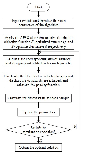
the initial power of the electric vehicle. The specific flow of solving
the multi-objective optimization problem based on the APSO algorithm is
shown in Figure 2.
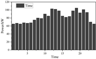
The daily load curve of a building is used for simulation verification, and the data are shown in Figure 3, which shows that the average daily load power of the power grid is 82.875 kW. For the convenience of calculation, it is assumed that 2,000 EVs of the same model are connected to the power grid, with driving consumption power of 8 kW, rated battery capacity of 40 kW/h, and maximum charging and discharging power of 15 kW, and the initial charge state of the incoming EV is 0.8, and the minimum charge state of outgoing EV is 0.9, which is required by users. The initial charging state of EVs entering the station is 0.8, and the minimum charging state of EVs leaving the station required by users is 0.9.
Based on the data in Figure 3, according to the mathematical model mentioned above and the set parameters, the effect of adjusting the load profile of the basic particle swarm algorithm and the adaptive particle swarm algorithm proposed in this paper is verified using MATLAB simulation software, respectively. Figure 4 shows the load exchanged between EVs and the grid, and the hourly average exchanged loads of the APSO algorithm and the PSO algorithm are 2.7092 P/kW, respectively, 1.9979 P/kW.
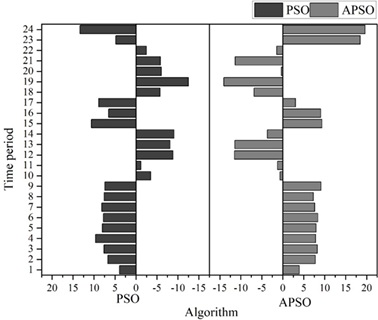
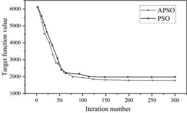
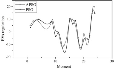
Figure 5 shows the change curve of the number of iterations of the objective function value, as can be seen from Figure 5, the objective function value decreases with the increase of the number of iterations until the maximum number of iterations can be reached to obtain the optimal solution, the improved PSO algorithm iteration speed as well as the attained fitness function value are better than before, and the iteration speed is close to 0 when the objective function value is 1809.The regulation amount of Figure 5 is counted in the grid and Figure 6 shows the EVs regulation amount, the peak regulation effect of these two algorithms is compared, the APSO algorithm is slightly higher than the PSO algorithm, and at the four peaks of 9:00, 16:00, 20:00, and 23:00, the regulation amount of the APSO algorithm is 9.638, 9.955, -1.584, and 19.819 are higher than the PSO algorithm, respectively.
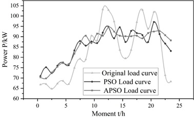
The regulated amount of Figure 6 is counted into the grid and the peak regulation effect of these two algorithms is compared, and Figure 7 shows the peak load curve of the grid, from which it can be seen that the original load curve is in the load trough period from 23:00 to 6:00, while two load peaks occur at 12:00 to 14:00 and 19:00 to 22:00. Simulation results show that the technique in this paper basically realizes the coordinated control of microgrid power and achieves the effect of peak shaving and valley filling, in which the improved algorithm has a significant improvement over the original grid state, indicating that the algorithm is superior to the basic particle swarm algorithm, and the daily load curve can be almost replaced by a constant load curve, and for the two peaks of load occurring at 12:00\(\mathrm{\sim}\)14:00 and 19:00\(\mathrm{\sim}\)22:00 , the power is stabilized between 89.184 P/kW to 94.514 P/kW. This is of great benefit to the power distributor and also reduces the price of electricity, bringing convenience to the customer.
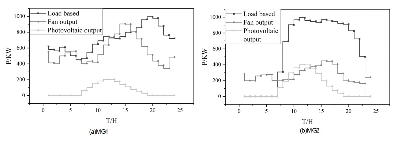
The wind turbine output, PV output, and base load of the microgrid system are shown in Figure 8, with MG1 in Fig. 8(a) and MG2 in Figure 8(b), where MG1 and MG2 denote the community and park microgrids, respectively, and the two MGs have the same ESS storage parameters, with the capacity of 1500 kW/h, the maximum charging and discharging power of 225 kW, and the maximum, minimum, and initial state of charge of 0.9, 0.3, respectively, 0.5, and the charging/discharging efficiency is 0.9. The base loads of the community and the park are different, the base load of the community is maintained at 453.05 P/KW\(\mathrm{\sim}\)995.48 P/KW all day long, and the base load of the park is 0 P/KW for two time periods, from 1:00 to 7:00 and from 20:00 to 24:00.
In order to analyze the influence of different weight coefficients on the optimization results, Figure 9 shows the comparison of the optimization results with different weight coefficients, comparing the optimization results under five groups of different weight coefficients, in which the values of weight coefficient 1 are taken as 0, 0.3, 0.5, 0.8, and \(\lambda _{1}\) in the groups, and the weight coefficients \(\lambda _{2}\) are taken as 1, 0.7, 0.5, 0.2, and 0, respectively. And based on the optimization results, the integrated operation and management costs and load fluctuation variance of microgrids in one dispatch cycle are counted.
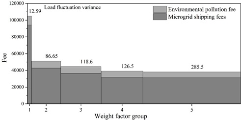
Setting different weight coefficients will have an impact on the optimization results, and when the weight coefficient \(\lambda _{1}\) increases, the microgrid operation cost and environmental pollution cost gradually decrease, while the load fluctuation variance increases with the decrease of the weight coefficient \(\lambda _{2}\). In order to select the appropriate weight coefficients so that the microgrid operation and management costs and environmental pollution control costs, as well as load fluctuation variance and other indicators to achieve the optimal operating state, first of all, to obtain the optimization results of the model under the single-objective, i.e., to select the operating results of array 1 and array 5 in Figure 9, to obtain the maximum value of the microgrid operation and management costs, environmental pollution control costs, as well as the load fluctuation variance are respectively 94056.856\(\mathrm{\yen}\), 10765.096\(\mathrm{\yen}\), and 285.469, and the minimum values are 31195.564\(\mathrm{\yen}\), 6945.064\(\mathrm{\yen}\), and 12.585, respectively.Then, the entropy weight method is applied to calculate the weight coefficients of each objective function, and the weight coefficients \(\lambda _{1}\) and \(\lambda _{2}\) are 0.578 and 0.422, respectively.Finally, the weight coefficients obtained are applied to weight the different objective functions. Finally, applying the obtained weighting coefficients to weight different objective functions, the proposed model is solved, and the microgrid operation and management cost, environmental pollution cost and load fluctuation variance are 319654.468\(\mathrm{\yen}\), 7694.954\(\mathrm{\yen}\) and 120.594, respectively.
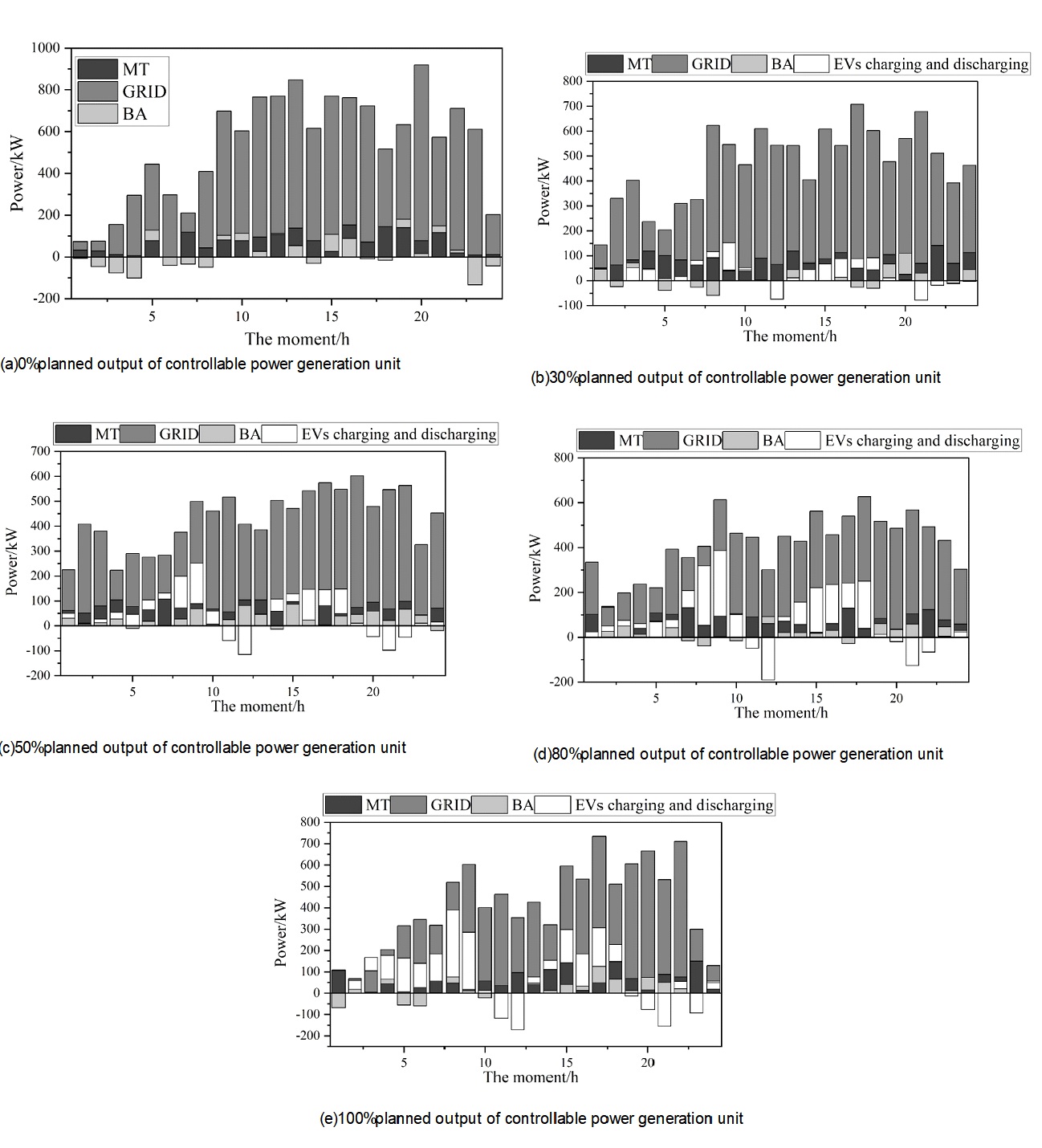
To study the power output of controllable generating units with different responsiveness, the user responsiveness in the region is selected as 0%, 30%, 50%, 80%, and 100%, and the operation results are shown in Figure 10, and the integrated operation and management costs of microgrids with different user responsiveness in 1 dispatch cycle are counted, and Figure 10(a)-(e) are 0%, 30%, 50%, 80%, and 100%, respectively. In the figure, MT is the microfuel engine, BA is the energy storage system, and GRID is the power curve of the public power grid. Table 1 shows the comparison of microgrid metrics with different user responsiveness.
From the change of power supply to the public power grid in Figure 10(a), it can be seen that the scaled EVs are connected to the microgrid in an uncontrolled manner during the 8:00-20:00 time period, and the power load of the microgrid rises sharply in the peak hours of electricity demand, which results in the increase of the power supply from the public grid to the microgrid, with the power range between 400 and 1000 kW, which is prone to put the public power grid in an overloaded state. The power range is between 400\(\mathrm{\sim}\)1000kW, which is easy to make the public power grid in overload state. When the user response degree is between 30% and 80%, with the increase of user response degree, the operation and management cost of microgrid and the cost of environmental pollution control are reduced accordingly, the operation and management cost and the cost of environmental pollution control are reduced from 37,564.185 yuan to 28,618.439 yuan, and from 8,765.515 yuan to 7,864.685 yuan, respectively, and the load fluctuation is reduced. The variance has a tendency to decrease and then increase. At 100% user responsiveness, large-scale EVs are connected to the regional microgrid for charging and discharging, and due to the limitation of the installed capacity of distributed energy resources in the regional microgrid, the demand for electricity in the region increases, resulting in a corresponding increase in the costs associated with the microgrid, and at the same time, the load fluctuation variance increases compared to that at 50% and 80% responsiveness.
| Responsiveness /% | Microgrid operating costs \(\mathrm{\yen}\) | Environmental pollution control costs \(\mathrm{\yen}\) | Load fluctuation variance \(\mathrm{\yen}\) |
| 0 | 45466.698 | 9465.168 | 254.945 |
| 30 | 37564.185 | 8765.515 | 146.698 |
| 50 | 31648.864 | 7896.451 | 114.489 |
| 80 | 28618.439 | 7864.685 | 134.544 |
| 100 | 35497.515 | 7916.648 | 194.748 |
In this paper, starting from the type and charging mode of electric vehicles and driving characteristics, we explore the influencing factors affecting the charging load of electric vehicles, construct a patterned EVs scheduling model, and put forward the microgrid operation optimization strategy as well as the constraints, taking into account the user response conditions. Adaptive particle optimization algorithm is used to solve the model.
Simulation example analysis is used to simulate and verify the daily load profile of the test site, and the average daily load of the microgrid based on the patterned EVs scheduling optimization model is obtained as 82.875 kW. According to the mathematical model and the set parameters, the effects of adjusting the load profile of the basic particle swarm algorithm and the adaptive particle swarm algorithm proposed in this paper are verified respectively, and the time-averaged exchange loads of the APSO algorithm and PSO algorithm are 2.70%, 2.7% and 2.7% respectively. The average exchange load of APSO algorithm and PSO algorithm are 2.7092 P/kW and 1.9979 P/kW respectively, and the effect of APSO algorithm is better than PSO.
To study the power output of controllable power generation units with different user responsiveness, when the user responsiveness is 0%, the scaled EVs are connected to the microgrid in an uncontrolled manner during the 8:00-20:00 time period, and the power supplied to the microgrid from the public power grid is also increased, and the power range is in the overloaded state between 400 and 1000 kW. And when the user responsiveness is between 30% and 80%, the operation and management cost and the environmental pollution control cost decrease from 37564.185 yuan to 28618.439 yuan and 8765.515 yuan to 7864.685 yuan, respectively, and the cost is effectively reduced.