
Population development is a strategic issue related to peace and development in today’s world, and all major issues in the process of modernization are closely related to population development [16, 4]. As the most populous developing country in the world, China’s population is always a major issue affecting comprehensive, coordinated and sustainable development, and a key factor constraining economic and social development [17, 12, 8]. Therefore, effective and accurate prediction of China’s future population size is of great significance to the country’s continuous promotion of economic and social development and progress as well as the realization of the strategy of comprehensive human development [18, 1]. At present, there are a large number of literature studies on China’s population growth, but most of them are based on the overall level of China’s population without considering the specific conditions of China, i.e., there are differences between urban and rural areas in terms of medical care, sanitation, education, and the economy, and these differences will inevitably lead to the different characteristics of births and deaths of the urban and rural populations [14, 3, 13, 23].
China is a populous country, and the population problem has always been one of the key factors constraining China’s development [21, 7]. It is an important issue to make analysis and prediction of China’s population based on the available data and using mathematical modeling. In recent years, China’s population development has shown some new characteristics, such as the accelerated aging process, the continuous increase in the sex ratio at birth, and the urbanization of the rural population, all of which affect the growth of China’s population [11, 20, 6]. Population forecasting is accomplished by collecting basic information, building forecasting models and determining forecasting parameters, among other basic aspects [19]. There are more basic methods and models for population forecasting, and the more popular and practical ones are generally age shift algorithms, matrix equations, population development equations and exponential equations [15, 22]. Population development equation is a new set of population forecasting model proposed by Chinese scholar and famous expert of the end-of-control-century era system theory, Song Jianyu, in the late 1970’s. This set of population forecasting model has the ability to predict the population of the country in the future. This set of prediction model has the advantages of more reasonable setting of prediction variables, more careful consideration of prediction parameter factors, and easy to be generalized and applied [10, 5, 2]. Therefore, this set of prediction models is the most popular and widely used set of population prediction models in China today [9]. At the same time, this set of prediction models has also had a great influence outside China.
The population development equation is composed of a series of matrix equations: \[\label{GrindEQ__1_} \left\{\begin{array}{l} {X^{s} \left(t+1\right)=H^{s} \left(t\right)X^{s} \left(t\right)+\left[1\; 0\; \cdots \; 0\right]^{T} \eta _{0A} \left(t\right)y^{s} \left(0\right)_{t} +W^{s} \left(t\right)^{T} X^{s} \left(t\right)} ,\\ {y^{s} \left(0\right)_{t} =\beta \left(t\right)S^{s} \left(t\right)F^{{\rm T}} \left(t\right)X^{{\rm f}} \left(t\right)} .\end{array}\right. \tag{1}\]
The above equation represents the forecast model for the population aged above zero, while the following equation describes the forecast model for the population aged zero. The superscript \(s\) denotes gender, where \(s=m\) represents males and \(s=f\) represents females \(F^{T} \left(t\right)\) is the transpose of the fertility pattern matrix \(F\left(t\right)\),and \(\beta \left(t\right)\) represents the total fertility rate for year \(t\). \(S^{s} \left(t\right)\) is the birth sex ratio; \(\eta _{0A} \left(t\right)\) represents the infant survival rate for year \(t\), and \(y^{s} (0)_{t}\) denotes the number of newborns by gender in year \(t\).
\(X^{s} \left(t\right)=\left[\begin{array}{l} {X^{s} \left(0,t\right)} \\ {X^{s} \left(1,t\right)} \\ {\quad \cdots } \\ {X^{s} \left(M,t\right)} \end{array}\right]\) is the age-specific population vector, where \(X^{s} \left(k,t\right)\) represents the number of individuals aged \(k\) by gender in year \(t\), with \(k=0,1,\cdots ,M\) and \(M\) representing the maximum age. \[\label{GrindEQ__2_} H^{s} \left(t\right)=\left[\begin{array}{ccccc} {0} & {\cdots } & {\cdots } & {0} & {0} \\ {1-d_{0} } & {0} & {\cdots } & {0} & {0} \\ {0} & {1-d_{1} } & {0} & {\vdots } & {\vdots } \\ {\vdots } & {\vdots } & {\ddots } & {0} & {0} \\ {0} & {0} & {\cdots } & {1-d_{M-1} } & {0} \end{array}\right], \tag{2}\] is the population survival rate matrix for year \(t\),where \(d_{k}\) represents the age-specific mortality rate, which can be calculated as \(d_{k} =\frac{D_{k} }{X_{k} }\),where \(D_{k}\) is the number of deaths at age \(k\), and \(X_{k}\) is the total population at age \(k\), with \(k=0,1,\cdots ,M\),and \(M\) being the maximum age.
The equation \(W^{s} \left(t\right)=\left[\begin{array}{c} {IR\left(0,t\right)} \\ {IR\left(1,t\right)} \\ {\vdots } \\ {IR\left(M,t\right)} \end{array}\right]\) represents the age-specific migration rate vector, where \(IR\left(k,t\right)\) is the migration rate for the population aged \(k\) in year \(t\).This can be calculated as: \[\label{GrindEQ__3_} IR\left(k,t\right)=\frac{hx_{k}^{\left(t\right)} -hx_{k}^{\left(t-1\right)} }{x_{k} } , \tag{3}\] where \(hx_{k}^{\left(t\right)}\) is the retained population of age \(k\) in year \(t\),and \(hx_{k}^{\left(t-1\right)}\) is the retained population of the same age in the previous year \(t-1\), with \(k=0,1,\cdots ,M\), and \(M\) being the maximum age.
The matrix \(F^{T} \left(t\right)=\left[\begin{array}{ccccccccc} {0} & {\cdots } & {0} & {f^{s} \left(\begin{array}{c} {\vartheta ,t} \end{array}\right)} & {\cdots } & {f^{s} \left(\begin{array}{c} {\xi ,t} \end{array}\right)} & {0} & {\cdots } & {0} \end{array}\right]\) represents the transpose of the fertility pattern vector. Here, \(f^{{\rm s}} \left(\varepsilon ,t\right)\) denotes the normalized age-specific fertility rate, with \(\vartheta\) and \(\xi\) representing the minimum and maximum ages of the fertility cycle, where \(\vartheta \le \varepsilon \le \xi .\)
When using the above population development model for population forecasting, the ability to reasonably preset parameters such as mortality patterns, fertility patterns, fertility levels, and population migration rates is critical to the accuracy of the forecast results. In previous population forecasts, these indicators were often given simple assumptions or fixed at values from a particular time period. However, with improvements in productivity levels and the refinement of healthcare systems, fertility and mortality patterns are dynamically changing. Additionally, uneven development of urbanization across regions has led some areas to approach the limits of urbanization or even experience reverse urbanization. Therefore, parameter presetting should utilize big data processing techniques for dynamic identification in order to better reflect population changes.
Multilayer Perceptron (MLP) and Random Forest (RF) are two types of machine learning algorithms, which will be discussed in Sections 2.2.1 and 2.2.2 respectively. To enhance the performance of both algorithms, stacking techniques are employed to combine them, resulting in the MLP-RF stacking model. Stacking is an ensemble learning technique that allows the development of an integrated model starting from multiple regression, linear regression, or classification models. Specifically, the original dataset is first divided into a training set and a validation set. Single models, such as decision trees, neural networks, or support vector machines, are developed on the training dataset. The validation dataset is then used to make predictions using the base models, and the predictions are treated as new features, known as meta-features, which constitute a second-layer dataset or meta-dataset.
Next, using the meta-dataset, a meta-learner is employed to further develop the ensemble model. In this study, Reptile is selected as the meta-learner. Reptile was proposed by researchers at OpenAI in 2018, and its core idea is to optimize model parameters by simulating “transfer” across a distribution of tasks. It utilizes a simple gradient descent process, training the base models across several different tasks. For each task, a few gradient descent updates are performed, and then the updated parameters are averaged and compared with the original data. This process yields a gradient pointing towards an “average task,” allowing for quick learning of new tasks.
The specific steps of the Reptile algorithm are as follows:
1) Initialization: Randomly initialize model parameters \(\theta ;\)
2) Task Sampling: Sample a batch of tasks \(T_{i}\) from the task distribution \(P\left(T\right)\). In this context, the tasks can be understood as different objective functions in the regression problem;
3) Inner Loop Update: For each task \(T_{i}\), extract a mini-batch of data \(D_{i}\) from its dataset. Use the data \(D_{i}\) to perform several gradient descent updates on the model parameters \(\theta\), resulting in new parameters \(\theta ';\)
4) Outer Loop Update: Compute the average of the new parameters \(\theta '\) obtained from all tasks, yielding a new parameter \(\theta _{new}\). Update the original parameters \(\theta\) as \(\theta \leftarrow \theta +\) \(\left(\theta _{new} -\theta \right)\).This step can be considered as an averaged update across multiple tasks;
5) Repeat Steps 2-4: Continue the update process until the model parameters converge or the predetermined number of iterations is reached.
The Multilayer Perceptron (MLP) is a special type of feedforward neural network, also known as a deep feedforward network. It consists of a layered architecture composed of interconnected nodes or neurons, as illustrated in Figure 1. Its structure comprises three different layers: the input layer, the hidden layer(s), and the output layer. The input layer consists of a set of neurons corresponding to the input variables, and one or more hidden layers contain a certain number of neurons. Each node in the figure represents a neuron, and its input-output relationship can be expressed by Eq. (4): \[\label{GrindEQ__4_} y=h\left({\mathop{\sum }\limits_{j}} \omega _{j} x_{j} +b\right). \tag{4}\]
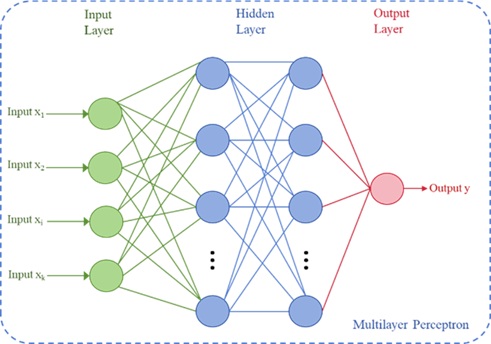
In the formula, \(y\) represents the output value of the neuron, \(x_{j}\) denotes the input value of the neuron, \(h\left(x\right)\) is the activation function, \(\omega _{j}\) represents the weight of the connection between nodes, and \(b\) is the bias value. These neurons perform nonlinear transformations on the data in the hidden layers using weighted linear combinations and nonlinear activation functions. As a result, the weight values and biases are optimized at each layer. The output from each hidden layer is continuously passed to subsequent layers until the final predicted result reaches the output layer.
The training of a multilayer perceptron involves the backpropagation algorithm, a technique used to minimize the loss function. The training samples are labeled, meaning their output values are known. The randomly initialized feature values of the samples are fed as inputs to the neural network, and through forward computation, the network produces output values. By comparing the network’s predicted values with the true output values of the samples, the weights and biases of each layer in the network are adjusted backward to minimize the loss function. Ultimately, the neural network learns to automatically derive the relationship between input and output.
The Random Forest algorithm is an ensemble prediction technique based on decision trees. It constructs multiple decision trees for classification or regression, and makes coherent predictions for the target variable by means of voting or averaging. The working process is shown in Figure 2. Each decision tree consists of a root node with a training dataset, internal nodes where conditional states are set based on input variables, and leaf nodes that represent the actual values assigned to the target variable.
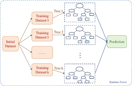
The construction of the decision tree model primarily involves recursively dividing the input dataset into subsets. The prediction value for each subset is generated using a multivariable linear regression model. Then, by continuously splitting the subsets into smaller branches, the model evaluates all potential splits within each field to promote the iterative growth of the tree. This step can be understood as finding an optimal, near-optimal, or even suboptimal split point within the tree’s subsets, increasing tree diversity while ensuring relatively optimal results. In the iterative process, least-squares deviation is used for the subdivisions. \[\label{GrindEQ__5_} R\left(t\right)=\frac{1}{N\left(t\right)} {\mathop{\sum }\limits_{i\in t}} \left(y_{i} -y_{m} \left(t\right)\right)^{2} . \tag{5}\]
In the formula, \(R\left(t\right)\) represents the error value at each node, \(N\left(t\right)\) denotes the number of units at the node, \(y_{i}\) represents the value of the target variable in the \(i\)-th unit, and \(y_{m}\) is the mean value of the target variable at node \(t\). The algorithm will stop when \(R\left(t\right)\) reaches its minimum or when it meets certain stopping criteria.
In regression tasks, each decision tree outputs a continuous value as its prediction, and the final prediction is the average of all the tree outputs. Using the collective opinions of multiple decision trees improves prediction accuracy, enhances the robustness of the model, and reduces the risk of overfitting that can occur in multilayer perceptions.
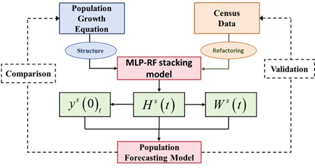
Based on the mathematical form of the population development equation, it is clear that the key challenges and crucial points in population prediction lie in the calculation and estimation of indicators such as the population retention matrix, population transition matrix, and fertility pattern vector. The critical point in calculating the population retention matrix \(H^{s} \left(t\right)\) is the prediction of population mortality levels. By relying on data from the sixth and seventh national population censuses, and selecting highly correlated input and output data, the MLP-RF algorithm is utilized for deep learning to establish a gender- and age-specific retained population model. On the basis of the population retention matrix, the population transition matrix \(W^{s} \left(t\right)\) can be calculated and predicted by computing the difference between the retained population in year \(t\) and the retained population in year \(t-1\). At the same time, by predefining the age range of women of childbearing age and using the MLP-RF model to predict the retained population data by gender and age, the population data of women of childbearing age can be obtained. Then, by using the MLP-RF algorithm to identify the mathematical model between the population of women of childbearing age and the newborn population, newborn population predictions can be made. The process of population prediction based on the population development equation and the MLP-RF model is shown in Figure 3.
The data used are sourced from the 2010 Sixth National Population Census, the 2020 Seventh National Population Census, and population sampling data from 2010 to 2020. The population data of Hebei Province is selected as the case study. First, by combining the total population, birth rate, and natural growth rate from the two population censuses, the total population and mortality data by gender and age over a 10-year period (2010–2019) are organized and estimated. Next, based on the population sampling data, the difference between the retained population in year \(t\) and year \(t-1\) is calculated to obtain the population migration data. Finally, the population data of childbearing age (15-64 years old) by gender and age, as well as the population data of newborns (0 years old), are selected to train the fertility model \(y^{{\rm s}} (0)_{t}\). The specific data are shown in Tables 1 to 3. Due to the large volume of data, only the data and structure for a particular year are displayed:
| Age | population | Population of male | Population of female | Death of male | Death of female |
| 0 | 1136461 | 610587 | 525874 | 13614 | 10591 |
| 1\(\sim\)4 | 4007713 | 2150553 | 1857162 | 5806 | 3602 |
| 5\(\sim\)9 | 4256974 | 2266152 | 1990823 | 1997 | 684 |
| 10\(\sim\)14 | 3302628 | 1757199 | 1545429 | 837 | 248 |
| 15\(\sim\)19 | 5203889 | 2651943 | 2551946 | 1528 | 566 |
| 20\(\sim\)24 | 7566465 | 3759012 | 3807454 | 3403 | 1565 |
| 25\(\sim\)29 | 5946704 | 2962997 | 2983709 | 2550 | 1280 |
| 30\(\sim\)34 | 4857325 | 2473781 | 2383544 | 2359 | 1083 |
| 35\(\sim\)39 | 5174753 | 2609815 | 2564939 | 3632 | 1695 |
| 40\(\sim\)44 | 6297435 | 3186559 | 3110873 | 6759 | 3128 |
| 45\(\sim\)49 | 5739783 | 2871820 | 2867962 | 9123 | 4462 |
| 50\(\sim\)54 | 4704672 | 2396406 | 2308268 | 12814 | 6319 |
| 55\(\sim\)59 | 4809622 | 2419612 | 2390011 | 21456 | 11300 |
| 60\(\sim\)64 | 3431129 | 1714407 | 1716722 | 25803 | 15141 |
| 65\(\sim\)69 | 2091111 | 1042786 | 1048325 | 24425 | 15662 |
| 70\(\sim\)74 | 1605949 | 798255 | 807695 | 31995 | 24143 |
| 75\(\sim\)79 | 1154141 | 536189 | 617952 | 32467 | 30901 |
| 80\(\sim\)84 | 616417 | 262379 | 354039 | 24802 | 32052 |
| 85\(\sim\)89 | 232813 | 87265 | 145548 | 11858 | 21144 |
| 90\(\sim\)94 | 54655 | 17725 | 36929 | 3121 | 7984 |
| 95\(\sim\)99 | 10397 | 3142 | 7254 | 503 | 2023 |
| 100+ | 1029 | 210 | 819 | 134 | 361 |
| Year | Population of birth | |
| Male | Female | |
| 2010 | 610587 | 525874 |
| 2011 | 640956 | 562687 |
| 2012 | 668327 | 586990 |
| 2013 | 624125 | 548179 |
| 2014 | 634893 | 557826 |
| 2015 | 481812 | 423508 |
| 2016 | 587883 | 516649 |
| 2017 | 574494 | 504940 |
| 2018 | 466805 | 410400 |
| 2019 | 424051 | 372905 |
| 2020 | 360685 | 317216 |
| Age | Population of male | Population of female | Migration of male | Migration of female |
|---|---|---|---|---|
| 0 | 596973 | 515283 | 7353 | 6390 |
| 1\(\sim\)4 | 2144747 | 1853560 | -6384 | -2639 |
| 5\(\sim\)9 | 2264155 | 1990139 | -3167 | 1184 |
| 10\(\sim\)14 | 1756362 | 1545181 | 465 | 3594 |
| 15\(\sim\)19 | 2650415 | 2551380 | -12640 | -10655 |
| 20\(\sim\)24 | 3755609 | 3805889 | -47531 | -42293 |
| 25\(\sim\)29 | 2960447 | 2982429 | -41404 | -29896 |
| 30\(\sim\)34 | 2471422 | 2382461 | -30849 | -19798 |
| 35\(\sim\)39 | 2606183 | 2563244 | -26551 | -14518 |
| 40\(\sim\)44 | 3179800 | 3107745 | -19467 | -10100 |
| 45\(\sim\)49 | 2862697 | 2863500 | -8878 | -427 |
| 50\(\sim\)54 | 2383592 | 2301949 | -7549 | 1370 |
| 55\(\sim\)59 | 2398156 | 2378711 | -16377 | -4178 |
| 60\(\sim\)64 | 1688604 | 1701581 | -20046 | -10103 |
| 65\(\sim\)69 | 1018361 | 1032663 | -20664 | -13014 |
| 70\(\sim\)74 | 766260 | 783552 | -27658 | -22069 |
| 75\(\sim\)79 | 503722 | 587051 | -30078 | -30853 |
| 80\(\sim\)84 | 237577 | 321987 | -22927 | -31150 |
| 85\(\sim\)89 | 75407 | 124404 | -10527 | -19115 |
| 90\(\sim\)94 | 14604 | 28945 | -2678 | -6747 |
| 95\(\sim\)99 | 2639 | 5231 | -508 | -1294 |
| 100+ | 76 | 458 | -6 | -3 |
Note: For ease of display, except for the population data of ages 0 and over 100, the rest of the age groups are displayed in 5-year intervals.
Based on the predicted values from the model and the validation dataset, an error analysis is conducted to evaluate the model’s performance. In this study, the evaluation metrics used are the Coefficient of Determination (R²), Root Mean Squared Error (RMSE), and Mean Absolute Error (MAE). The specific descriptions of the evaluation metrics are as follows:
| Error analysis function | Mathematical formulas | Performance evaluation |
|---|---|---|
| \(R^{2}\) | \(R^{2} =1-\frac{\sum\limits_{i=1}^{n} \left(X_{P}^{i} -X_{M}^{i} \right)^{2} }{\sum\limits_{i=1}^{n} \left(\overline{X_{M} }-X_{M}^{i} \right)^{2} }\) | The proportion of the dependent variable’s variability explained by the independent variables in the regression model, evaluating the goodness of fit between the data and the model. |
| RMSE | \(RMSE=\sqrt{\frac{\sum\limits_{i=1}^{n} \left(X_{P}^{i} -X_{M}^{i} \right)^{2} }{n} }\) | The square root of the total squared error between the predicted results and the validation dataset, which is highly sensitive to large prediction errors. |
| MAE | \(MAE=\frac{\sum\limits_{i=1}^{n} \left|X_{P}^{i} -X_{M}^{i} \right|}{n}\) | The absolute error between the predicted results and the validation dataset, describing the accuracy of the model’s predictions. |
In the Table 4, \(X_{M}^{i}\) represents the actual value of the population at age \(i\), \(X_{P}^{i}\) represents the predicted value of the population at age \(i\), \(\overline{X_{M} }\) is the average population across all ages, and \(n\) is the maximum age range of the population. Here, \(n\) is set to 100 or the specified number of age groups.
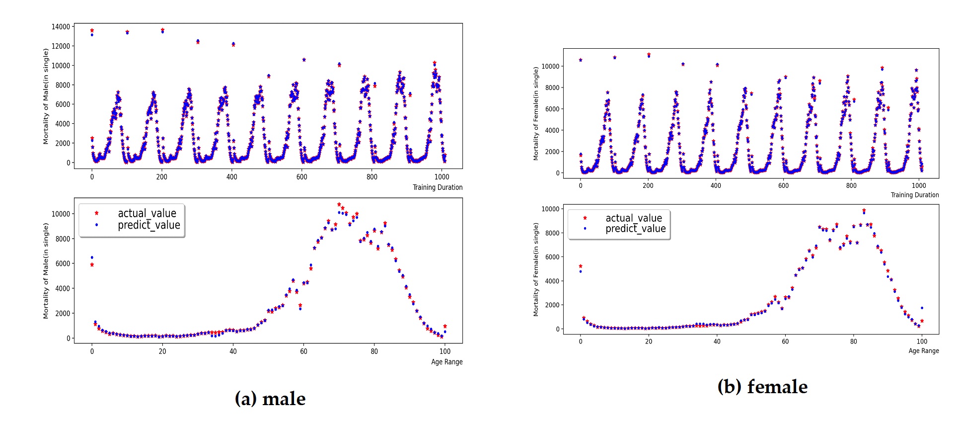
When training the retention population model by gender and age group, we first perform regression training on the total population and the deceased population. The training parameters in the MLP and RF models are set respectively. The hidden_layer represents the number of hidden layers in the MLP, which is set to (400, 600) here. Max_iter refers to the maximum number of iterations, set to 2000. alpha represents the regularization strength coefficient to prevent model overfitting, set to 0.001. solver refers to the algorithm used to solve optimization problems, where the LBFGS (Limited-memory Broyden Fletcher Goldfarb Shanno) algorithm is selected. random_state is used to initialize the random number generator’s state, set to 0 here. learning_rate_init indicates the initial learning rate of the model, set to 0.01. n_estimators represents the number of trees in the Random Forest, set to 10,000. max_depth refers to the maximum depth of the trees, set to 100. n_jobs represents the number of parallel processors used, set to 6. min_samples_split is an important parameter in the Random Forest, controlling the minimum number of samples required to split a node, set to 2. min_samples_leaf controls the minimum number of samples required in a leaf node, set to 1.
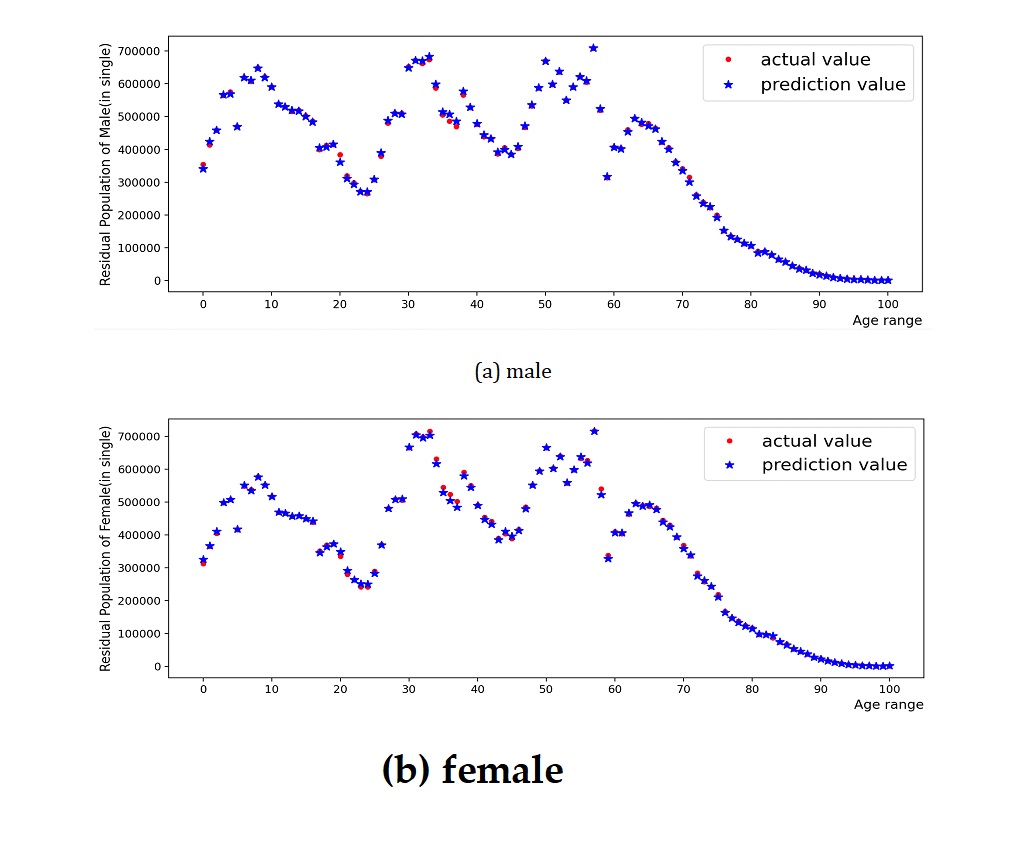
Figure 4 and Figure 5 present the training process and prediction results of the total population and deceased population by gender and age group. The model was trained using population data from 2010 to 2019, and population predictions for 2020 were obtained. Using the natural retention population matrix, the retention population by gender and age group, as shown in Figure 6, was obtained. The model was evaluated using an error function, where the for the male retention population model was 0.998, the RMSE was 10515.3, and the MAE was 6974.3. For the female retention population model, the was 0.997, the RMSE was 10932.4, and the MAE was 7641.8. This indicates that the MLP-RF stacked model has a high prediction accuracy for the retention population, with relatively small root mean square error and mean absolute error, suggesting that there are few instances of significant deviation in the prediction results.
The migration population model by gender and age group uses parameters similar to those used in the retention population model during the training process. In the migration population model, the parameter is added to control decision tree pruning. The study used population migration data from Hebei Province from 2010 to 2018, and obtained population migration prediction data for 2019, as shown in Figure 7.
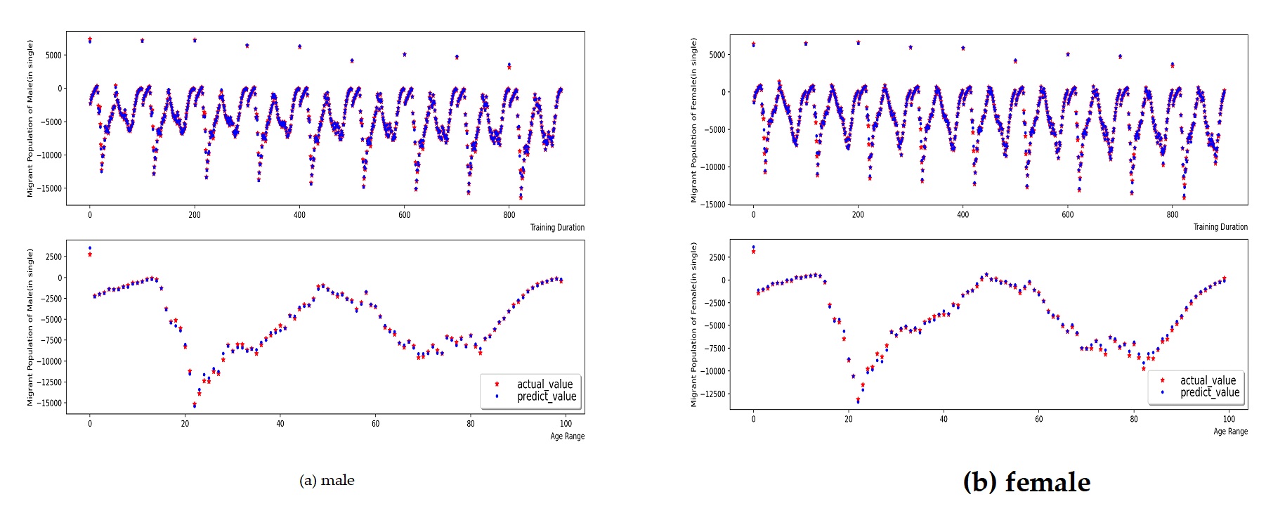
By calculating the error function of the predicted data, it is found that the \(R^{2}\) of the male migrant population model is 0.995, RMSE is 255.43, and MAE is 189.07; the \(R^{2}\) of the female migrant population model is 0.999, RMSE is 266.70, and MAE is 197.43. Error analysis results show that the MLP-RF stack model is still very accurate in predicting the transfer population, especially the female transfer population, and the reason for the relatively simplified composition of the transfer population data cannot be ruled out. Subsequently, multi-source mobile communication data can be introduced for model training, which can more truly reflect the migration and flow state of the population.
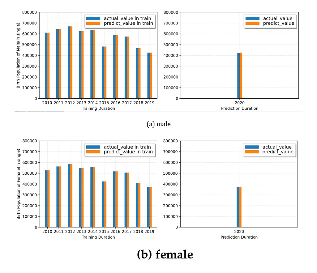
The gender-specific birth population prediction model was trained using gender- and age-specific population data from 2010 to 2019. The population aged 15 to 64 was defined as the reproductive population, while the population aged 0 was used as the birth population data. In addition to the previously mentioned model parameters, this model also included settings for min_weight_fraction_leaf, max_samples, min_impurity_decrease, and ccp_alpha. These settings constrain the sample weight proportion for the leaf nodes of the decision tree, the number of base model samples, and the minimum reduction in node impurity.
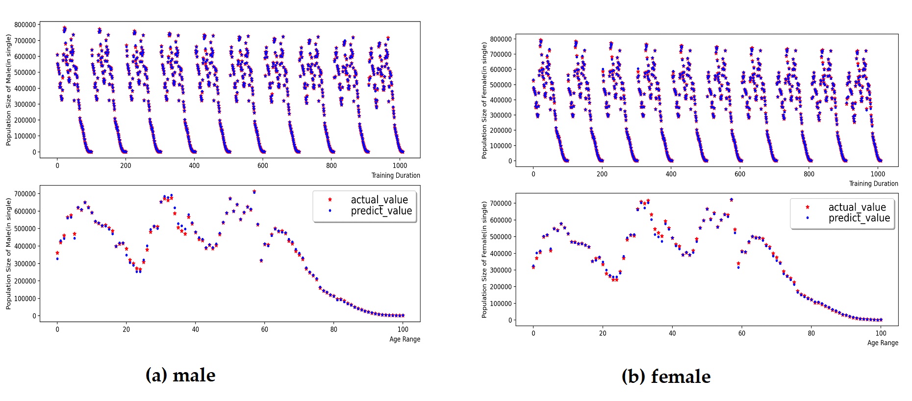
Figure 8 shows the training process and prediction results of the birth population model by gender. The predicted male birth population deviates from the actual value by 1,035, with a mean absolute percentage error (MAPE) of 0.29%. The predicted female birth population deviates from the actual value by 1,021, with a MAPE of 0.33%. Based on these results, it can be concluded that the stacked model achieves high accuracy in predicting both male and female birth populations.
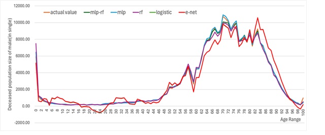
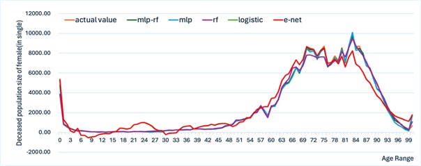
In section 3 , the stacked model of multi-layer perceptron and random forest along with the population development equation was employed to predict the population. Does this combined prediction model have an advantage in fitting accuracy compared to other commonly used prediction models? This paper selected four approaches, namely the statistical model (Logistic), the linear regression model (Elastic-Net), the individual multi-layer perceptron, and the random forest algorithm, to train and predict the death population model and the transfer population model in population prediction, and conducted a comparative analysis with the prediction results of the MLP-RF combined prediction model.
The training process and prediction results of the contrastive prediction algorithm for the death population by gender and age are depicted in Figure 9 Figure 12. Through the calculation and analysis of the error function (Table 5 to Table 6), it can be observed that the Logistic model and the Elastic-Net model exhibit a poor degree of fit. This is attributed to their utilization of linear assumptions for data identification and the presence of multi-collinearity issues in the population data, leading to a significant over-fitting phenomenon in the 0-45 age range and a larger total error of the data. The MLP model and the RF model have a better degree of fit, indicating that these two models possess a stronger ability to identify data. Nevertheless, the MLP-RF stacked model has a relatively better degree of fit and a smaller data error, suggesting that the stacked model integrates the advantages of the two machine learning models and enhances the prediction accuracy of the population data.
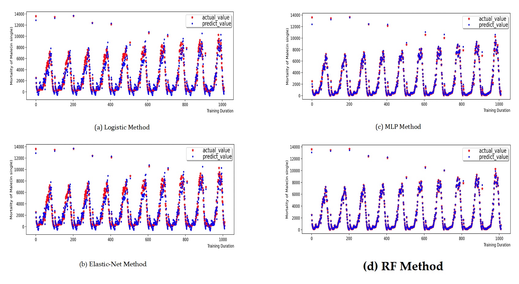
| \(R^{2}\) | RMSE | MAE | |
|---|---|---|---|
| MLP-RF | 0.998 | 142 | 84 |
| Logistic | 0.951 | 753 | 590 |
| Elastic-Net | 0.951 | 752 | 589 |
| MLP | 0.998 | 138 | 92 |
| RF | 0.993 | 267 | 145 |
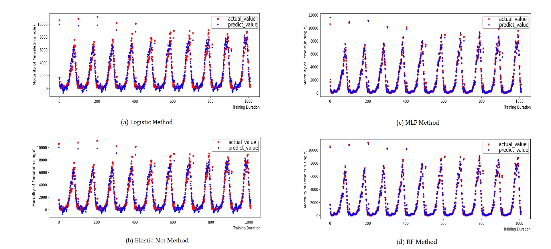
| \(R^{2}\) | RMSE | MAE | |
|---|---|---|---|
| MLP-RF | 0.998 | 150 | 72 |
| Logistic | 0.955 | 648 | 495 |
| Elastic-Net | 0.955 | 647 | 493 |
| MLP | 0.997 | 167 | 96 |
| RF | 0.993 | 258 | 124 |
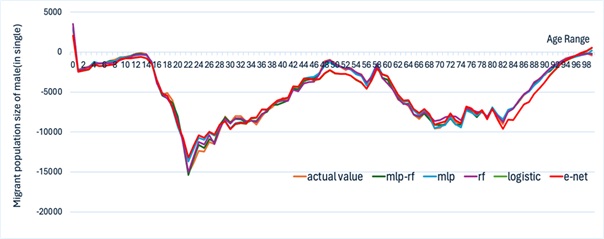
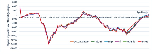
Figure 13 to Figure 16 present the training process and prediction results of each contrastive prediction algorithm for the migrant population by gender and age. In conjunction with the graph curves and the calculation and analysis of the error function (Table 5 to Table 6), it can be verified that the MLP-RF stacked model has more advantages in predicting the migrant population compared to traditional statistical models, linear regression models, and standalone machine learning models.
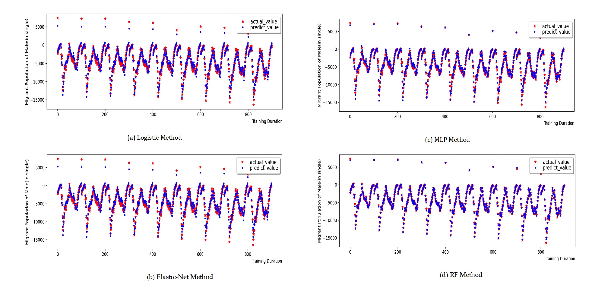
| \(R^{2}\) | RMSE | MAE | |
|---|---|---|---|
| MLP-RF | 0.995 | 255 | 189 |
| Logistic | 0.956 | 768 | 615 |
| Elastic-Net | 0.956 | 766 | 613 |
| MLP | 0.981 | 498 | 342 |
| RF | 0.991 | 332 | 226 |
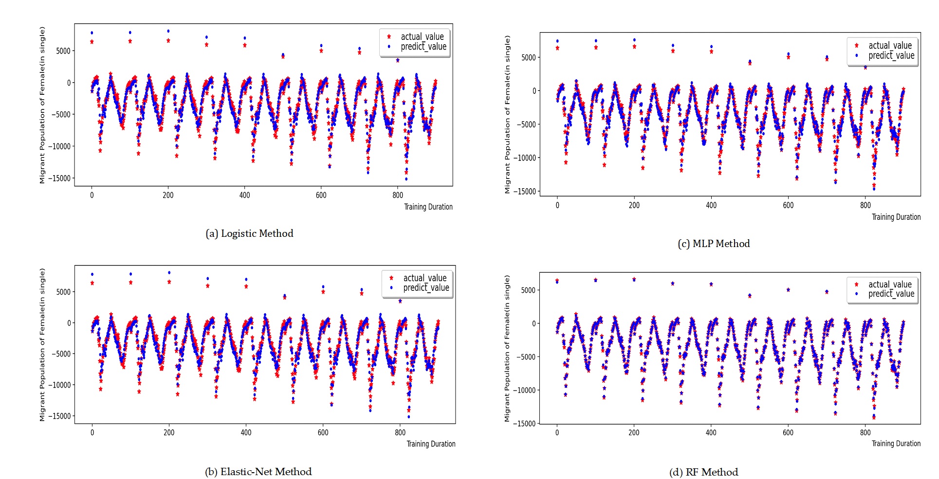
| \(R^{2}\) | RMSE | MAE | |
|---|---|---|---|
| MLP-RF | 0.999 | 267 | 197 |
| Logistic | 0.993 | 696 | 565 |
| Elastic-Net | 0.993 | 695 | 564 |
| MLP | 0.996 | 537 | 433 |
| RF | 0.998 | 285 | 176 |
This study is based on a discrete population development equation and a stacked model of two machine learning algorithms, Multilayer Perceptron (MLP) and Random Forest (RF).The population data of the Sixth Population Census and the Seventh National Population Census were reconstructed to obtain the population data of Hebei Province by gender and age from 2010 to 2020, and the model training and prediction of the deaths, retained populations, migrant populations and births of Hebei Province by sex and age were carried out. This study addresses the following technical challenges:
1) Data reconstruction: To ensure the data met the operational requirements of the discrete population development equation, the census data were reconstructed by gender and age using annual population sampling data and other statistical sources. This approach significantly expanded the training dataset’s capacity and addressed the issue of insufficient data size.
2) Model Integration: The integration process involved addressing the coupling effects on parameter design within the two models. A reptile meta-learner was employed to facilitate this integration. Through extensive debugging sessions, the design of key parameters for both models was finalized, allowing the complementary strengths of the two algorithms to enhance the overall performance of the integrated model.
By analyzing and comparing the forecasting models, the following key conclusions can be drawn:
1) Using the discrete population development equation as the basic prediction model, the MLP-RF stacked model was employed to identify and predict parameters such as the natural retention rate and birth rate, which would otherwise need to be manually preset. This approach not only considers the internal statistical mechanisms of population change but also avoids prediction errors caused by preset parameters to some extent.
2) According to the prediction results, the MLP-RF stacked model achieved high accuracy in predicting retention population, migration population and birth population. The model showed good fitting results for population counts across different genders and age groups. However, the census data used for model training still has some problems, such as single source and poor real-time performance, which makes it impossible to give full play to the ability of machine learning model for large-scale data processing. Future research could address this by incorporating larger datasets with more diverse sample types and more real-time mobile communication data, providing strong support for migration population predictions.
The integration of multiple machine learning models into a new stacked model shows promising results for population prediction, particularly in analyzing age- and gender-specific population structures and forecasting mortality and birth rates. With the development of mobile communication data, the stacked model has a strong potential for large-scale data training and prediction.
This work was supported by Soft Science Research Project of Innovation Ability Improvement Plan in Hebei Province (Grant number: 23556103D).