
Power systems based on the Internet of Things (IoT) mainly use devices such as smart meters, transformer monitors, voltage and current sensors, etc., to monitor the operating status of the power system in real time, and to take relevant measures to ensure the efficient and stable operation of the system by collecting detailed power quality data such as voltage, current, frequency and power [24, 1]. Abnormalities in power quality data often occur due to equipment failures, sensor errors, communication interruptions and data transmission errors. This not only affects the real-time monitoring and control of the power system, but also leads to a reduction in the operational efficiency of the power system and errors in decision-making. Traditional data restoration methods, such as mean padding and linear interpolation, fail to make full use of the spatial and temporal correlation of data, and although they are simple and direct, they can only handle a small amount of missing data. Moreover, the mean padding method leads to the loss of dynamic change characteristics of the data, and the linear interpolation method is seriously inadequate in repairing accuracy when facing complex nonlinear data [7]. Matrix filling is a method of inferring unknown elements by known elements when some elements of the matrix are missing, which is widely used in the fields of recommender systems, image processing and signal processing [12]. This method takes into account the correlation between data and can repair the missing data more effectively.
In the study of power quality data restoration, in order to improve the restoration accuracy, singular value decomposition and low rank approximation algorithms were used for optimisation to assist in filling in the missing values on the results after column mean filling. The optimisation incorporates alternating least squares and kernel paradigm minimisation for iterative optimisation to further enhance the repair results. After verifying the filling effect through cross-validation and error assessment metrics, the results show that the method exhibits high accuracy at low missing rates and outperforms the traditional algorithm. In addition, the SVD algorithm can show higher accuracy and stability after combining the methods of kernel-paradigm minimisation and gradient descent for the repair effect. It can be seen that the method provides a systematic data preprocessing and filling process, which provides a new technical means for repairing anomalous and missing data in the power system.
This article is divided into five main parts: the first part is the introduction, which introduces the problem of missing data and its importance in the power IoT; the second part is related work, which summarizes the existing data restoration methods and their limitations; the third part describes the proposed data restoration system in detail, including the specific methods and steps of data preprocessing, matrix filling, and result validation; and the fourth part is the experimental results and analysis. The effectiveness of the proposed method is verified through comparison and ablation experiments, and the contribution of each component to the overall performance is analyzed; the fifth part is the conclusion, which summarizes the research results, points out the shortcomings of the research, and proposes future research directions.
In recent years, various methods have been proposed to improve the accuracy and efficiency of power quality data restoration, among which the commonly used methods are statistical modelling and interpolation. Chen [4] investigated the method of combining 5G communication technology with distributed computing to enhance the performance of power IoT, which improves the system efficiency and security by optimising the data transmission and processing. Gaddam, et al. [8] proposed a hybrid model-based data consistency approach to solve the problem of data inconsistency in heterogeneous power IoT systems. Singh et al. [23] investigated smart home energy management system using IEEE 802.15.4 and Zigbee protocols for data transmission in order to improve the efficiency of data collection and processing. Ismail et al. [13] proposed a smart grid data restoration method based on Wireless Sensor Network (WSN), which improves the accuracy of data restoration by combining machine learning algorithms. Teh et al. [26] studied the use of statistical methods for sensor data restoration, which significantly improved the effectiveness of data restoration. Although these methods have to some extent solved the problem of data repair, they still have shortcomings in dealing with large-scale data loss and utilizing data correlation.
In order to address the issues in existing research, many scholars have explored different data restoration methods. Chaurasia et al. [3] proposed an IoT assisted wireless sensor network optimization method based on metaheuristic algorithm, which improves data transmission efficiency and accuracy by improving routing protocols. Senthil et al. [21] studied a hybrid particle swarm optimization algorithm applied to energy-efficient cluster routing to optimize the data repair process. Prasanth and Jayachitra [18] proposed a multi-objective optimization strategy to enhance the data repair performance of IoT enabled WSN (Internet of Things-enabled Wireless Sensor Network) applications by improving service quality. Ramalingam et al. [19] studied a hybrid optimization algorithm for cluster routing protocols in information center wireless sensor networks, which improved the robustness of data restoration. Sharma et al. [22] proposed an energy sensitive routing framework that combines machine learning and metaheuristic algorithms, effectively improving the accuracy of IoT data restoration. Although these methods have made some progress in improving the efficiency and accuracy of data restoration, they still have limitations in handling complex data missing patterns and utilizing spatiotemporal correlations. Therefore, this article studies a method based on low rank matrix filling algorithm to more effectively handle large-scale data loss and improve the accuracy and efficiency of data repair.
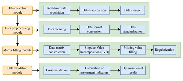
This study investigates the power quality data restoration system for the Internet of Things based on the low rank matrix filling algorithm. The data collection module, data preprocessing module, matrix filling module, and data verification module of the system were designed. Among them, the data collection module is responsible for collecting power quality data in the power Internet of Things. The data preprocessing module cleans and formats the collected data. The matrix filling module applies low rank matrix filling algorithm to repair missing data. The data validation module evaluates and optimizes the repair results. Figure 1.
As shown in Figure 1, the system architecture consists of four main modules: a data collection module that collects, transmits, and stores real-time power quality data; the data preprocessing module performs data cleaning, format conversion, and standardization; the matrix filling module constructs a data matrix, applies SVD to fill missing values in the data, and performs regularization processing; the data validation module calculates evaluation indicators through cross validation and displays the repair results. These modules work together to achieve efficient and accurate restoration of power quality data.
To ensure the accuracy and completeness of power quality data, a series of specific methods and techniques have been adopted in the data collection module. The data is collected from multiple monitoring points within a certain residential area, with each monitoring point recording data for one month, covering key parameters such as voltage, current, frequency, etc. Table 1 shows the tools and related environments used in the data collection process.
| Serial number | Tool Name | Function | Brand or Model | Deployment Location |
| 1 | Smart meter | Record voltage, current, etc. | Schneider Electric ION7650 | Monitoring Point |
| 2 | Voltage sensor | Detect voltage transients, sags, and swells | Fluke 435 Series II | Monitoring Point |
| 3 | Current sensor | Detect current harmonics and imbalance | Yokogawa CW500 | Monitoring Point |
| 4 | Frequency meter | Monitor grid frequency | Keysight 53220A | Monitoring Point |
| 5 | Distributed database system | Data storage and management | Apache Cassandra | Data Center |
| 6 | Hadoop distributed file system | Large-scale data storage | Apache Hadoop | Data Center |
| 7 | Kafka message queue | Real-time data synchronization | Confluent Kafka | Data Center |
In Table 1, the instruments and equipment used in the data collection process are recorded. Among them, numbers 1-4 record the equipment used for detecting and recording power quality parameters, while numbers 5-7 record the software used for data transmission and storage. Table 1 provides a brief introduction to the names, functions, models, and corresponding deployment environments of these devices, which can help staff understand the device information for data collection and accelerate the data collection process.
In terms of data collection, high-frequency data collectors are used for real-time monitoring of power quality parameters, and each monitoring point is equipped with smart meters, voltage sensors, current sensors, and frequency meters. Among them, the voltage records the effective voltage value, peak voltage value, voltage transient, voltage dip, and voltage rise events of each phase. The current records the effective value of the current, current harmonics, and current imbalance. The frequency records the grid frequency and frequency deviation. All devices undergo strict calibration and validation to ensure the reliability of data. Data collection includes multiple cycles to ensure high-frequency and low latency data acquisition, meeting the needs of real-time monitoring. Table 2 shows some of the raw data collected during the acquisition phase, which provides a high-quality data foundation for subsequent data preprocessing and matrix filling.
As shown in Table 2, the power quality data of ten monitoring points in the power Internet of Things are listed. Monitoring points 1 to 10 record the effective value of the voltage, the total harmonic voltage distortion (THDu), the effective value of the current, the total harmonic current distortion (THDi), the current unbalance degree, the line frequency, and the waveform distortion rate. These data points reflect the power quality characteristics of the grid at different locations. The effective voltage fluctuation range is between 229.8V and 231.2V, indicating the stability of the power grid voltage; The effective current value is between 14.6A and 15.5A, indicating the variation of the load. These data are crucial for analyzing the operational status of the power grid, but in actual operation, there may be missing or abnormal data, which affects the accuracy of data analysis. Therefore, matrix filling-based methods are adopted to repair these missing or abnormal data, ensuring the stable operation of the power IoT monitoring and control system. This process not only enhances the accuracy of data, but also ensures the continuity and reliability of power system monitoring, providing solid data support for the power Internet of Things.
In terms of data transmission, two methods, 5G network and wired network, have been adopted to ensure real-time and stable data transmission. For data storage, Hadoop Distributed File System (HDFS) is used for data storage [15]. HDFS divides the collected data into a number of data blocks, each of which is stored independently, thus ensuring efficient data storage. A redundant storage strategy is used to store copies of data blocks on multiple nodes to improve data reliability and availability.
| Monitoring point | Voltage effective value (V) | THDu (%) | Current effective value (A) | THDi (%) | Current unbalance degree (%) | Line frequency (Hz) | Wave form distortion (%) |
| 1 | 230.5 | 3.5 | 15.2 | 4.1 | 2.5 | 50 | 2.9 |
| 2 | 231 | 3.8 | 14.8 | 4.3 | 2.8 | 49.9 | 3 |
| 3 | 229.8 | 3.6 | 15.5 | 4 | 2.6 | 50.1 | 2.8 |
| 4 | 230.2 | 3.7 | 14.9 | 4.2 | 2.7 | 50 | 2.9 |
| 5 | 230.7 | 3.6 | 15 | 4.1 | 2.6 | 50 | 3 |
| 6 | 231.1 | 3.5 | 14.7 | 4.3 | 2.5 | 49.9 | 2.8 |
| 7 | 229.9 | 3.7 | 15.3 | 4 | 2.7 | 50.1 | 2.9 |
| 8 | 230.3 | 3.6 | 14.8 | 4.2 | 2.6 | 50 | 3 |
| 9 | 230.6 | 3.8 | 15.1 | 4.3 | 2.8 | 50 | 2.8 |
| 10 | 231.2 | 3.9 | 14.6 | 4.4 | 2.9 | 49.9 | 2.9 |
To ensure data quality and consistency, a data quality monitoring module is integrated to monitor data integrity and accuracy in real time. Data consistency checking algorithm is used to compare real-time collected data with historical data to detect and mark abnormal data. Real-time data synchronisation is achieved using Kafka message queues to transmit the collected data to multiple storage nodes in real-time [5]. A combination of incremental and full backups is used to ensure that the data can be recovered in case of system failure or accident. Among them, incremental backup records the data changes since the last backup, and full backup backs up all the data periodically.
Median and low-pass filters are used in data cleaning to filter noise from the collected data [16, 10]. The median filter effectively removes spiky noise by replacing the values of data points with the median of their neighboring data. Assuming the original data sequence is \(x=\left\{x_{1} ,x_{2} ,\ldots ,x_{n} \right\}\), the data \(y=\left\{y_{1} ,y_{2} ,\ldots ,y_{n} \right\}\) processed by the median filter can be represented as: \[\label{GrindEQ__1_} y_{i} =median\left(x_{i-k} ,\ldots ,x_{i} ,\ldots ,x_{i+k} \right) . \tag{1}\]
Among them, k is the size of the filtering window. The mathematical expression for a low-pass filter is: \[\label{GrindEQ__2_} y_{i} =\alpha x_{i} +\left(1-\alpha \right)y_{i-1} . \tag{2}\]
Among them, \(\alpha\) is the smoothing coefficient, and 0\(\mathrm{<}\)\(\alpha\)\(\mathrm{<}\)1. Outlier detection uses box-and-line plot method and 3\(\sigma\) method to identify and remove outlier data [28, 17]. Quartiles, means and standard deviations of the data were calculated to identify and remove outliers exceeding 1.5 times the interquartile spacing and outliers exceeding three times the standard deviation range.
Data format conversion is the second step of preprocessing and aims to unify data formats from different sources. The data from different sources were uniformly converted to CSV (Comma-Separated Values) format to ensure the consistency of data structure. The linear interpolation method is used to time-align the data from different collection frequencies to ensure the synchronisation of the data at each monitoring point. The formula for linear interpolation is: \[\label{GrindEQ__3_} y\left(t\right)=y\left(t_{0} \right)+\left(\frac{y\left(t_{1} \right)-y\left(t_{0} \right)}{t_{1} -t_{0} } \right)\left(t-t_{0} \right) . \tag{3}\]
Among them, \(y\left(t\right)\) is the data point to be estimated, \(y\left(t_{0} \right)\) and \(y\left(t_{1} \right)\) are known data points, and \(t_{0}\) and \(t_{1}\) are the timestamps of known data points.
Data standardization is the final step of preprocessing, which converts data of different dimensions into the same dimension to eliminate the influence of dimensions between data. In this process, the z-score standardization method is mainly used to standardize the data [20]. For each data point, its standard score can be calculated by subtracting the mean of the data and then dividing by the standard deviation of the data. In this way, the data is transformed into a standard normal distribution with a mean of 0 and a standard deviation of 1. This not only eliminates the dimensional influence of data, but also enhances the convergence and stability of the algorithm. After preprocessing, the raw data is presented as the data in Table 3.
| Voltage effective value | THDu | Current effective value (A) | THDi | Current unbalance degree | Line frequency | Wave form distortion |
| -0.0164 | -0.6283 | 0.8198 | 0 | -0.9045 | 0 | 0 |
| 0.6691 | 0.9425 | -1.1488 | 1 | 0.9045 | -1.4252 | 1.4142 |
| -1.1751 | -0.2094 | 1.6397 | -1 | -0.3015 | 1.4252 | -1.4142 |
| -0.6529 | 0.1616 | -0.8198 | 0.5 | -0.6029 | 0 | 0 |
| 0.3365 | -0.2094 | 0 | 0 | -0.3015 | 0 | 1.4142 |
| 1.0046 | -0.6283 | -1.6397 | 1 | -0.9045 | -1.4252 | -1.4142 |
| -0.9838 | 0.1616 | 0.8198 | -1 | -0.6029 | 1.4252 | 0 |
| -0.4916 | -0.2094 | -1.1488 | 0.5 | -0.3015 | 0 | 1.4142 |
| 0.1752 | 0.9425 | 0.4099 | 1 | 0.9045 | 0 | -1.4142 |
| 1.3044 | 1.3613 | -2.0496 | 1.5 | 1.5075 | -1.4252 | 0 |
In Table 3, the preprocessed power quality data are presented, which are sourced from raw measurements of power IoT monitoring points. Before entering the matrix filling algorithm, they undergo Z-score normalization to eliminate dimensional effects and centralize data distribution. The standardized data presents a distribution around zero values, such as the effective voltage value ranging from -1.1751 to 1.3044, which represents the degree of deviation of the voltage level at the monitoring point relative to the average value. Similarly, the standardized value of THDu ranges from -0.6283 to 1.3613, reflecting the deviation of the distortion degree of the voltage waveform at each monitoring point relative to the average distortion. For the effective value of current, the standardized values range from -2.0496 to 1.6397, indicating the fluctuation of current intensity. In addition, the normalised data for THDi, current unbalance, line frequency and waveform distortion rate reveal the complexity of the current waveforms, the balance of the three-phase currents, the stability of the grid frequency and the fluctuating characteristics of the overall power quality, respectively.
In this study, the relevant repair of preprocessed power quality data is achieved by using a low-rank matrix filling algorithm to ensure the completeness and accuracy of the data [14]. This section describes in detail the specific steps of matrix filling, which are divided into data matrix construction, SVD decomposition, low-rank approximation, initial filling, iterative optimisation and regularisation process in the order of before and after [9, 2].
The matrix construction stage involves forming the preprocessed data into a matrix form and producing the experimental data matrix required for the experiment according to different data missing rates in order to complete the subsequent experiments. When determining the basic parameters of the matrix required for the experiment, the row and column information of the matrix needs to be determined according to the temporal and spatial characteristics of the data. The number of rows n can be selected based on the ratio of the total collection time to the collection time interval. According to the number of monitoring points, the number of columns m can be determined to obtain the original data matrix of n rows and m columns. Then, the data in the evidence can be randomly extracted with data loss rates of 10%, 20%, …, and 80% to create corresponding experimental samples. These samples are used to verify the repair effect of the matrix filling method in power quality data.
To achieve the method of repairing data using matrix filling, this article adopts the SVD method to decompose the data matrix, and constructs a low rank approximation matrix through screening to reveal the inherent structure of the data and provide a basis for subsequent missing value filling. After the initial filling, the filling matrix is iteratively optimized, and after convergence, regularization is performed to further improve the filling effect, finally obtaining the required data matrix with complete data. The specific method steps are as follows:
By SVD decomposition, the original matrix is represented as the product of a set of singular values and their corresponding singular vectors, revealing the intrinsic structure of the data. The formula is: \[\label{GrindEQ__4_} A=U\Sigma V^{T} . \tag{4}\]
By using low rank approximation to reduce matrix complexity while preserving key information, simplifying the main features and structure of data, and providing a solid foundation for subsequent matrix filling processes, the formula is: \[\label{GrindEQ__5_} A_{r} =U_{r} \Sigma _{r} V_{r}^{T} . \tag{5}\]
Figure 2 visualizes the implementation of the SVD algorithm.
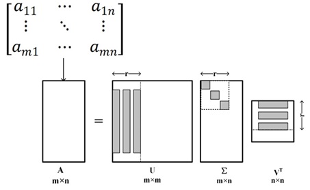
As shown in Figure 2, SVD decomposes matrix A into the product of three matrices. Among them, U is the left singular vector matrix of m\(\mathrm{\times}\)m, \({\rm \Sigma }\) is the diagonal matrix of m\(\mathrm{\times}\)n, containing singular values, and \(V^{T}\) is the right singular vector matrix of n\(\mathrm{\times}\)n. The low rank approximation constructs a low rank approximation matrix \(A_{r}\) with rank r by selecting and preserving the maximum r singular values and their corresponding singular vectors. Among them, \(U_{r}\) and \(V^{T}\) are the parts of U and V corresponding to the largest r singular values, respectively, and \({\rm \Sigma }_{r}\) is the corresponding diagonal matrix.
Missing values in the data matrix can be initially filled using the column mean filling method, replacing the missing values in each column with the mean of that column. The missing values can be ignored first to calculate the mean of each column of data, and then the mean can be used to fill in the missing values in the column, thus obtaining the preliminary filled matrix \(A_{init}\).
In order to optimise the matrix after initial padding, this study uses Alternating Least Squares (ALS) to optimise the matrix iteratively [11]. The objective function is constructed as follows: \[\label{GrindEQ__6_} {\mathop{\min }\limits_{V_{r} /U_{r} }} \left\| A-U_{r} \Sigma _{r} V_{r}^{T} \right\| _{F}^{2} . \tag{6}\]
Optimise the right singular vector matrix with fixed left singular vector and find the one that minimises the error by minimising this objective function. Similarly, optimise the left singular vector matrix with the right singular vector matrix fixed. By alternating these two steps, the optimisation continues so that the filled matrix gradually approaches the true matrix. Continue this process until the matrix converges, that is, the error between the filled matrix and the low-rank approximation matrix is minimised.
During the iterative optimisation process, the Nuclear Norm Minimization (NNM) constraint is introduced in this study in order to prevent the overfitting problem [29, 27]. The objective function is as follows: \[\label{GrindEQ__7_} {\mathop{\min }\limits_{A_{r} }} \left\| A-A_{r} \right\| _{F}^{2} +\lambda \left\| A_{r} \right\| _{*} \tag{7}\]
Among them, \(\left\| A_{r} \right\| _{*}\) represents the kernel norm of the matrix, which is the sum of all singular values, and \(\lambda\) is the regularization parameter. The parameters in the objective function are continuously adjusted to minimise the error between the filled matrix and the original matrix, but also to control the complexity of the matrix to prevent overfitting due to over-complexity of the model [30, 6]. In practice, the fitting error and model complexity are balanced by adjusting the regularisation parameter \(\lambda\).
The assessment metrics include Mean Squared Error (MSE), Mean Absolute Error (MAE), Root Mean Squared Error (RMSE) and Coefficient of Determination (R-squared, \(R^{2}\)) [25].
MSE is the average of the squared errors between the populated data and the true data, mathematically formulated as: \[\label{GrindEQ__8_} MSE=\frac{1}{N} \mathop{\sum }\limits_{i=1}^{N} (y_{i} -\hat{y}_{i} )^{2} . \tag{8}\]
MAE is the mean of the absolute errors between the populated data and the real data, corresponding to the equation: \[\label{GrindEQ__9_} MAE=\frac{1}{N} \mathop{\sum }\limits_{i=1}^{N} \left|y_{i} -\hat{y}_{i} \right| . \tag{9}\]
The RMSE is the square root of the mean of the sum of squared differences between the post-fill data and the true data, which is given by the formula: \[\label{GrindEQ__10_} RMSE=\sqrt{\frac{1}{N} \mathop{\sum }\limits_{i=1}^{N} (y_{i} -\hat{y}_{i} )^{2} } . \tag{10}\]
\(R^{2}\) is a reflection of the goodness of fit between the populated data and the real data and is calculated as: \[\label{GrindEQ__11_} R^{2} =1-\frac{\mathop{\sum }\nolimits_{i=1}^{n} (y_{i} -\hat{y}_{i} )^{2} }{\mathop{\sum }\nolimits_{i=1}^{n} (y_{i} -\bar{y})^{2} } . \tag{11}\]
In the above formula, N is the number of missing values, \(y_{i}\) is the true value, and \(\hat{y}_{i}\) is the filled value. MSE and RMSE can quantify the overall error level between the filled data and the real data, reflecting the overall accuracy of the filling method. MAE can intuitively display the average level of error filling, which helps to understand the actual performance of the filling effect. R² can evaluate the goodness of fit between the filled data and the real data, reflecting the robustness and stability of the filling method.
The experimental data comes from power quality monitoring data in a certain residential area, with a total of 1000 data points, and eight missing rate levels of 10%, 20%, 30%, 40%, 50%, 60%, 70%, and 80% are set respectively. Figure 3 shows the indicator data validated in the experiment.
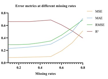
As shown in Figure 3, the data repair metrics are presented at different missing rates. These indicators are used to evaluate the effectiveness of matrix filling methods and help understand the degree of similarity between the repaired data and the original data. At a 10% missing rate, the values of MSE, MAE, and RMSE are approximately 0.1, 0.2, and 0.3, respectively. At a lower missing rate, the MSE is relatively small, indicating a better repair effect. As the missing rate increases, MSE gradually increases, which means that as the number of missing data increases, the difficulty of repair increases and the error also increases. In Figure 3, it was observed that R² reached 0.661 at a 10% missing rate. The closer R² is to 1, the better the repair effect, which means that the repaired data has a high degree of consistency with the original data.
In summary, although the difficulty of repairing increases with the increase of missing rate, matrix filling-based methods can still effectively restore missing data to a certain extent, especially at lower missing rates, where the repair effect is more significant. This also proves the effectiveness of the low rank matrix filling method in repairing power quality data. It is known that different missing rates can lead to different repair effects. To verify the impact of different sample sizes on repair errors, experimental results with 1000 and 2000 sample sizes are shown in Figure 4.
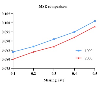
From Figure 4, it can be observed that as the missing rate increases, the MSE gradually increases for both 1000 and 2000 sample sizes, and the MSE for 2000 sample sizes is generally smaller than that for 1000 sample sizes. This indicates that under the same missing rate, the more abundant the sample size, the smaller the repair error in the experiment, and the better the data repair effect.
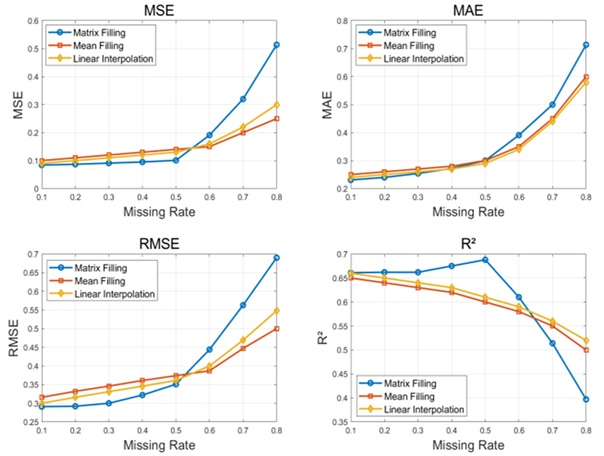
In order to verify the effectiveness of the low rank matrix filling algorithm in power quality data restoration, this article conducted comparative experiments with traditional mean filling and linear interpolation methods. The comparative experiment aims to evaluate the repair effectiveness of different data repair methods under different missing rates, using four evaluation indicators: MSE, MAE, RMSE, and R². The differences between these methods are shown in Table 4.
Table 4 shows some comparisons of the three methods. For each level of missing rate, mean imputation, linear interpolation, and low rank matrix imputation methods are used for data restoration. This article compares the repair effects of three methods at various missing rates, analyzes the advantages of low rank matrix filling methods, and evaluates the improvement level of indicators such as MSE, MAE, RMSE, and R². Figure 5 visually compares the error situation of three methods.
Figure 5 shows the repair effects of three methods based on low rank matrix filling, mean filling, and linear interpolation at different missing rates. It can be seen that before the loss rate of 0.5, the MSE, MAE, and RMSE based on the low rank matrix filling method are lower than the other two methods. After a missing rate of 0.5, the repair error of the low-rank matrix filling method gradually increases, and the repair effect is slightly insufficient compared with the other two traditional methods. This indicates that the low-rank matrix filling method can better retain the correlation between data when dealing with large-scale data missing problems at low missing rates, thus obtaining more accurate repair results. Besides, the R² indicator also shows that the fit of the low-rank matrix filling method is higher than the other two methods at 0.5 missing rate, indicating that it is more capable of restoring the real appearance of the original data. To sum up, the low-rank matrix filling method at low missing rate shows better performance in power quality data restoration and can be applied as an effective data restoration tool in the field of power IoT.
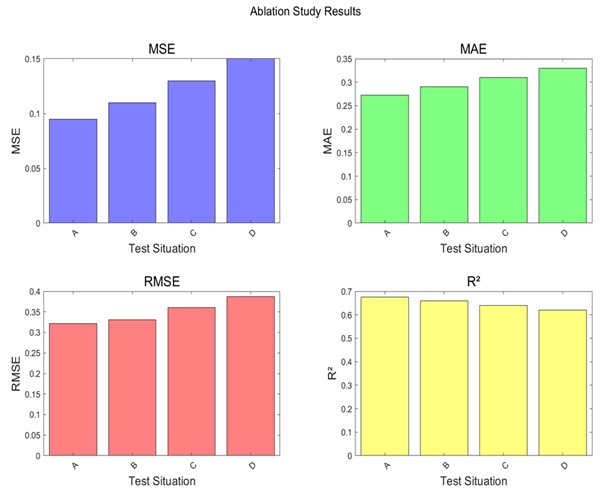
The effect of individual components on the overall performance can be visualised very well in ablation experiments. Four schemes were designed for the experiment:
1. Complete matrix filling method, including SVD, gradient descent, and kernel norm minimization.
2. Minimize the norm without kernel, using only SVD and gradient descent.
3. No gradient descent, using only SVD and kernel norm minimization.
4. Only SVD, without using gradient descent and kernel norm minimization.
Each scheme is tested at different missing rates and the changes in the four evaluation metrics of MSE, MAE, RMSE, and R² are recorded. The impact of each component on overall performance can be evaluated by comparing the experimental results of different schemes.
As shown in Figure 6, A, B, C, and D represent four scenarios: complete method, no kernel norm minimization, no gradient descent, and only SVD. When the missing rate is 40%, the MSE, MAE, RMSE, and R ² of the complete matrix filling are 0.095, 0.272, 0.322, and 0.675, respectively. When the nuclear free norm is minimized, they are 0.110, 0.290, 0.331, and 0.660, respectively. When there is no gradient descent, the values are 0.130, 0.310, 0.360, and 0.640, respectively. When only SVD is present, the values are 0.150, 0.330, 0.387, and 0.620, respectively. The experimental results show that the complete matrix filling method performs the best on all evaluation metrics, indicating that each component plays an important role in the data repair process. The removal of kernel paradigm minimisation and gradient descent processing in the component leads to a decrease in the restoration performance, especially in the MSE and R² metrics. The complete matrix filling method exhibits higher accuracy and stability in restoring power quality data.
This article proposes a power quality data repair system based on a low-rank matrix padding algorithm, which effectively handles the large-scale data missing problem in the Internet of Things (IoT) of electric power by using SVD, Alternating Least Squares (ALS), and kernel-paradigm minimisation. Experimental results show that the method exhibits high restoration accuracy and robustness at low missing rate, which is superior to the traditional mean padding and linear interpolation methods. The method not only improves the accuracy and efficiency of data repair, but also provides reliable data support for power system monitoring and control. Although the method in this article performs well in the experiments, there are still some shortcomings, such as higher computational complexity, which may consume more computational resources when dealing with large-scale data. The algorithm is more sensitive to the selection of parameters, which may need to be adjusted for different data sets to obtain the best results. Future research needs to combine new technologies such as deep learning to further improve repair effectiveness and algorithm efficiency, and promote the application of power quality data repair technology in smart grids and power Internet of Things. Considering the spatiotemporal correlation of power IoT data, the integration of spatiotemporal convolutional neural networks and other methods is also expected to make breakthroughs in improving data restoration effectiveness.