
Ringel [9] posed the famous Oberwolfach problem on the cycle decomposition of complete graphs. At conferences held in Oberwolfach, it is customary for participants to dine together at circular tables of varying sizes, with assigned seating that rearranges participants from meal to meal. The Oberwolfach problem asks how to make a seating chart for a given set of tables so that all the tables are full at each meal and all pairs of conference participants are seated next to each other exactly once. Formulated as a problem in graph theory, the pairs of people sitting next to each other at a single meal can be represented as a disjoint union of cycles of specified lengths, with one cycle for each of the dining tables. This union of cycles is a \(2\)-regular graph, and every \(2\)-regular graph has this form. If \(G\) is this \(2\)-regular graph with \(n\) vertices, the question is whether the complete graph \(K_n\) can be represented as an edge-disjoint union of copies of \(G\). In order for a solution to exist, the total number of conference participants (equivalently, the total number of vertices of the given cycles) must be odd. The problem has, however, also been extended to even values of \(n\) by asking whether all the edges of the complete graph, except a perfect matching, can be covered by copies of the given \(2\)-regular graph. Formally, the Oberwolfach problem \(OP(m_1^{\alpha_1},m_2^{\alpha_2},\ldots,m_t^{\alpha_t})\) asks for the existence of a \(2\)-factorization of a complete graph in which each \(2\)-factor consists of exactly \(\alpha_i\) cycles of length \(m_i\), for \(i=1,2,\ldots,t\). Much research has been done on this problem [1, 3, 2]. Gilbert [4] described cycle types of all lengths in \(Q_n\) for \(n\le 4\). Two paths in \(Q_n\) are said to have the same type if one path is obtained from the other by applying an automorphism. If no such automorphism exists between the two paths, then they are said to be distinct.
In this paper, we study the hypercube version of the Oberwolfach problem and obtain results related to cycle decompositions of hypercubes of even dimensions. We also develop an algorithm that generates all types of \(k\)-paths and hence \(k\)-cycles (since a cycle is a closed path) in \(Q_n\), where \(2\le k\le 2^n\) and \(n\ge 2\). Using the types of cycles, we give all possible cycle decompositions of \(Q_4\). We develop a technique for extending the cycle decomposition of \(Q_4\), together with a perfect matching, to the cycle decomposition of \(Q_6\), \(Q_8\), and, in general, \(Q_n\). We use properties of Cartesian products to extend \(2\)-factorizations of \(Q_4\) to factorizations of \(Q_8\), \(Q_{16}\), and so on.
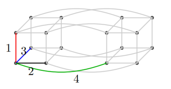
The vertices of \(Q_n\) are the binary \(n\)-tuples and two vertices are adjacent, if their corresponding \(n\)-tuples differ in exactly one co-ordinate. Let \(e_i=(0,\ldots 0,\underbrace{1}_{i^{th}~\textrm{place}},0,\ldots 0)\) be the standard unit vector, \(i\in \{1,2,\ldots,n\}.\) The direction of an edge \(e=(u,v)\) in \(Q_n\) is \(i,\) if \(u-v=e_i\) (subtraction is done modulo \(2\)).
A path \(P\equiv(u_1,u_2,\ldots,u_k)\) in \(Q_n\) can be expressed in terms of the initial vertex \(u_1\) and the edge direction sequence \(S=(i_1,i_2,\ldots,i_{k-1}),\) where \(i_j\in[n],\) such that for \(j=2,3,\ldots,k,\) \(u_j=u_1+\displaystyle \sum_{r=1}^{j-1}e_{i_r}.\) Similarly, a cycle \(C\equiv(u_1,u_2,\ldots,u_k,u_1)\) in \(Q_n\) can be expressed in terms of the initial vertex \(u_1\) and edge direction sequence \(S=(i_1,i_2,\ldots,i_k),\) where \(i_j\in\{1,2,\ldots,n\},\) such that for \(j=2,3,\ldots,k,\) \(u_j=u_1+\displaystyle \sum_{r=1}^{j-1}e_{i_r}\) and \(u_k+e_{i_k}=u_1.\) So the cycle \(C\equiv((0,0),(0,1),(1,1),(1,0),(0,0))\) in \(Q_2\) can be written as \(C((0,0),S),\) where \(S=(1,2,1,2).\)
In the following Figure 1, we have shown directions in hypercube \(Q_4.\)
Remark 2.1. If the initial vertex of a path is \(\textit{0},\) then the path is completely determined by its edge direction sequence. So, for convenience, we will represent a path \(P\equiv P(\textit{0},S),\) where \(S=(i_1,i_2,\ldots,i_k),\) by \(P=(i_1,i_2,\ldots,i_k)\) only.
The structure of \(Aut(Q_n)\) is well known. It is discussed in various articles ([4, 6, 8, 10]). There are two types of automorphisms complementation and permutation. Complementation refers to interchanging \(0\) and \(1\) in certain co-ordinate positions in the \(n\)-tuple. So it basically corresponds to the power set of \(\{1,2,\ldots,n\}.\) Suppose \(A\subseteq\{1,2,\ldots,n\},\) and \(\sigma_A\in Aut(Q_n)\) is the corresponding complementation. Then \(\sigma_A(x_1,x_2,\ldots,x_n)=(y_1,y_2,\ldots, y_n),\) where \[y_i=\left\{ \begin{array}{cc} x_i, & \textrm{if}~ i\notin A;\\ 1+x_i~(mod~2), & \textrm{if}~ i \in A. \end{array}\right.\]
However, permutation corresponds to the symmetric group \(S_n.\) For \(\theta\in S_n,\) \(\rho_{\theta}\in Aut(Q_n)\) is defined by \(\rho_{\theta}(x_1,x_2,\ldots,x_n)=(x_{\theta(1)},x_{\theta(2)},\ldots,x_{\theta(n)}).\)
Every element of \(Aut(Q_n)\) has a unique representation in the form \(\rho_{\theta}o\sigma_A.\) So \(|Aut(Q_n)|=2^n\cdot n!.\)
As hypercube is vertex-transitive, in our algorithm the paths have initial vertex \(\textit{0}=(0,0,0,\ldots,0).\) So only the edge-direction sequence will determine the path. Moreover, we use only permutations from \(Aut(Q_n)\) to check whether the types of a path are the same or distinct.
e.g.- (1) Consider paths \(P(\textit{0},S)\) and \(Q(\textit{0},S'),\) where \(S=(1,2,1)\) and \(S'=(3,4,3)\) in \(Q_4.\) Then there exists a permutation \(\theta=(1,3)(2,4),\) such that \(\theta(P)=Q.\) Therefore paths \(P\) and \(Q\) are of the same type.
(2) Suppose \(S'=(1,2,3)\) in the above example, then there does not exist an automorhism which will map \(P\) on \(Q.\) So \(P\) and \(Q\) are of different types.
Remark 2.2. Note that any two paths of length \(k\) are isomorphic, graph theoretically. But they can be of different type, depending upon their direction sequences. (See the e.g.(1) and (2) above.)
The algorithm which we write, constructs the edge-direction sequences of all possible types of paths in \(Q_n\) of length \(k,\) where \(n\geq 2\) and \(1\leq k \leq 2^n.\) It also identifies the closed paths, i.e., cycles from the edge-direction sequences. For this purpose, we construct binary matrices with \(n\) rows and \(k\) columns, \(1\leq k \leq 2^n.\) So if our path is \(P_k\equiv(\textit{0}=u_0,u_1,u_2,\ldots,u_k)\) of length \(k,\) then the matrix \(M_k\) corresponding to \(P_k\) will have \(n\) rows and \(k\) columns, where \(i^{th}\) column represents vertex \(u_i\) in the path, \(i=1,2,\ldots,k.\)
e.g.- Consider \(Q_4.\) Let \(P=P_6\) be a path of length \(6\) in \(Q_4,\) starting with vertex \(\textit{0}\) and having an edge direction sequence \((i_1,i_2,\ldots,i_6)=(1,2,3,4,1,3).\) Then the matrix corresponding to \(P\) will be as follows.
\[ M_{6} = \begin{array}{c} \begin{array}{@{}c@{\;}cccccc@{}} & \scriptstyle u_{1}&\scriptstyle u_{2}&\scriptstyle u_{3}&\scriptstyle u_{4}&\scriptstyle u_{5}&\scriptstyle u_{6} \end{array}\\[-0.4em] \left[ \begin{array}{cccccc} 1&1&1&1&0&0\\ 0&1&1&1&1&1\\ 0&0&1&1&1&0\\ 0&0&0&1&1&1 \end{array} \right] \end{array}. \]Observe that \(e_{i_j}=u_j-u_{j-1},\) for \(j=1,2,\ldots,6.\)
Recall that, in any path no two vertices are identical. As the columns of matrix under consideration correspond to vertices in a path, no two columns in the matrix are identical. Moreover, if the path is closed, i.e., if it is a cycle, then only the initial and final vertex are the same. So, here if a matrix corresponding to a path ends with \(\textit{0}\) vector, then we will get a cycle (as we are considering paths with initial vertex \(\textit{0}\)). Conversely, if one has a cycle with initial vertex \(\textit{0},\) then its corresponding matrix ends with a column containing all zeros.
e.g.- Consider a cycle \(C=(0,S),\) with \(S=(1,2,3,1,2,3),\) in \(Q_4.\) Then the corresponding matrix is
\[ M_{6} = \begin{array}{c} \begin{array}{@{}c@{\;}cccccc@{}} & \scriptstyle u_{1}&\scriptstyle u_{2}&\scriptstyle u_{3}&\scriptstyle u_{4}&\scriptstyle u_{5}&\scriptstyle u_{6} \end{array}\\[-0.4em] \left[ \begin{array}{cccccc} 1&1&1&0&0&0\\ 0&1&1&1&0&0\\ 0&0&1&1&1&0\\ 0&0&0&1&1&0\\ 0&0&0&0&0&0 \end{array} \right] \end{array}. \]So if a path is known, one can write a matrix corresponding to it. But then we have a question.
Question 2.3. In the given hypercube \(Q_n,\) where \(n\geq 2,\) is it possible to find all types of paths of length \(k,\) where \(1\leq k \leq 2^n,\) with the help of matrices?
Answer to the above question is yes and is given by our algorithm in the following subsection.
We prove a lemma before writing the algorithm.
Lemma 2.4. In a hypercube \(Q_n, ~n\geq 2,\) there exists only one type of path of length \(2,\) viz. \(P=(\textit{0},S),\) where \(S=(1,2)\) is the direction sequence.
Proof. Let \(Q=(v,S')\) with \(S'=(i_1,i_2)\) be an arbitrary path of length \(2\) in \(Q_n.\) We claim that \(P\) and \(Q\) are of the same type, i.e., there exists an automorphism (say) \(\phi \in Aut(Q_n),\) such that \(\phi(P)=Q.\)
If \(P=Q,\) there is nothing to prove.
Suppose \(P\neq Q.\) Then we have the following two cases.
Case 1. Suppose \(v=\textit{0}.\) Consider permutation \(\phi=(1,i_1)(2,i_2).\) Then \(\phi(P)=Q.\)
Case 2. Suppose \(v\neq\textit{0}.\) So let the \(n\)-tupple corresponding to \(v\) has \(1\)’s in the places \(i_1,i_2,\ldots,i_k,\) where \(V=\{i_1,i_2,\ldots,i_k\}\subseteq[n].\) Now consider the complementation \(\sigma_V,\) which will take \(\textit{0}\) to \(v.\) Now consider permutation \(\theta=(1,i_1)(2,i_2).\) Then \(\phi=\theta o \sigma_V\) is an automorphism of \(Q_n,\) such that \(\phi(P)=Q.\)
Hence the proof. ◻
Beacuse of the above lemma, for any path of length greater than \(2,\) its edge direction sequence will have the first entry \(1\) and the second entry \(2.\)
In our algorithm, we give a systematic way of generating paths of all types of a given length \(k\) in \(Q_n,\) using binary matrices of order \(n\times k,\) where \(2\leq k \leq 2^n\) and \(n\geq 2.\)
As all the paths generated in the algorithm have initial vertex \(\textit{0},\) here onwards, we denote path by the edge-direction sequence only. So if \(P\equiv P(\textit{0},S),\) where \(S=(1,2,1)\) is the edge-direction sequence, then we denote \(P\) as just \(P=(1,2,1).\)
Step 1. Initialization: We start with a binary matrix \(M_2=[u_1=e_1|u_2=e_1+e_2]_{n\times 2},\) which corresponds to the only type of path of length \(2,\) \(P_2=(1,2)=P\) (say). The idea is to extend \(P\) with the help of the matrix \(M_2.\) Note that the hypercube \(Q_n\) has the edges of directions from the set \([n].\) The path \(P\) has edges with directions \(1\) and \(2.\) So we call \(O=\{1,2\}\) as the old set for \(P.\) However, edges with directions \(3,\ldots,n\) are not present in \(P.\) So the set \(N=\{3,\ldots,n\}\) is referred as the new set for \(P.\)
(We give the immediate step for understanding below. One can skip the same and go to the Iteration step directly. Also note that, as there are no \(3\)-cycles in \(Q_n,\) possibility for cycle is not discussed in Step 2.)
Now for extending \(P,\) first consider the old set \(O\) corresponding to \(P.\) For every \(i\in O,\) construct a new matrix \(M_3^i=[M_2|u_2+e_i]\) of order \(n\times 3,\) by inserting a column at the end of \(M_2,\) which is a binary addition of the last column of \(M_2\) and \(e_{i}.\) Now we consider only those \(M_3^i\)’s which correspond to a path, i.e., no two columns of the matrix \(M_3^i\) are identical. We call those matrices as \(M_3^r,\) where \(r\in O\) gives a valid path.
Once all the elements in the old set of \(P_2\) are exhausted, we consider the new set \(N.\) In the new set of \(P,\) there are \(n-2\) elements. Consider the smallest element of \(N\) (say) \(s.\) Then construct a matrix \(M_3^s=[M_2|u_2+e_s].\)
So we get matrices \(M_3^r\)’s and a matrix \(M_3^s,\) which correspond to the valid path types of length \(3.\) Also note that the old set and new set for paths corresponding \(M_3^r\) are same as that of \(P,\) viz. \(O\) and \(N.\) However, the old set and the new set for path corresponding to \(M_3^s\) are \(O'=O\cup\{s\}\) and \(N'=N\setminus\{s\},\) respectively.
Step 3. Iteration: (i). Suppose there are \(d_{k-1}\) types of path of length \(k-1,\) viz. \(P_{k-1}^1,P_{k-1}^2,\ldots,\\P_{k-1}^{d_{k-1}},\) where \(3\leq k \leq 2^n.\) Let \(z_0=0\) and \(1\leq l \leq d_{k-1}.\)
Consider \(P_{k-1}^l.\) For convenience, call it \(P^l.\) Let \(M^l=[u_1|u_2|\ldots|u_{k-1}]\) be the corresponding matrix, \(O^l=\{i_1,i_2,\ldots,i_j\},\) \(j\leq k-1\) be the old set and \(N^l=[n]\setminus O^l\) be the new set for \(P^l.\) For every \(i_t\in O^l,\) construct a new matrix \(M^{l}(i_t)=[M^l|u_{k-1}+e_{i_t}]\) of order \(n\times k,\) by inserting a column at the end of \(M^l,\) which is a binary addition of the last column of \(M^l\) and \(e_{i_t}.\)
If any two columns in a matrix \(M^{l}(i_t),\) for some \(i_t\) are identical, then the direction sequence corresponding to the matrix \(M^{l}(i_t)\) does not represent a path. So it is not valid.
If the last column of a matrix \(M^{l}(i_t),\) for some \(i_t\) is identical to \(\textit{0}\) vector, then the direction sequence corresponding to the matrix \(M^{l}(i_t)\) is a cycle. Moreover, it can not be extended further.
So we consider only those \(M^{l}(i_t)\)’s which correspond to a path, i.e., no two columns of the matrix \(M^{l}(i_t)\) are identical for further expansion. Suppose there are \(z_l-1\) such matrices. So we rename those matrices as \(M^l_{k_r},\) where \(r\in \{z_{l-1}+1,z_{l-1}+2,\ldots,z_{l-1}+z_l-1\}.\) Here \(l\) in the superscript stands for \(P^l,\) \(k\) in the subscript stands for the type of path of length \(k.\) Also note that the old set and the new set for types corresponding to \(M^l_{k_r},\) where \(r\in \{z_{l-1}+1,z_{l-1}+2,\ldots,z_{l-1}+z_l-1\},\) are same as that of \(P^l,\) i.e., \(O^l\) and \(N^l\) respectively.
Once all the elements in the old set of \(P^l\) are exhausted, we consider the new set \(N^l.\) In the new set of \(P^l,\) there are \(n-j\) elements. Consider the smallest element of \(N^l\) (say) \(s.\) Then construct the matrix \(M^l(s)=[M^l|u_{k-1}+e_s]\) and call it as \(M^l_{k_{z_{l-1}+z_l}}.\) Now the old set and the new set for path corresponding to \(M^l_{k_{z_{l-1}+z_l}}\) are \(O'=O^l\cup\{s\}\) and \(N'=N^l\setminus\{s\},\) respectively.
So we get matrices \(M^l_{k_{r}}\)’s, where \(z_{l-1}+1\leq r \leq z_{l-1}+z_l,\) which correspond to the valid path types of length \(k\) obtained from \(P^l.\) For convenience, we call these matrices as \(M_k^r,\) and corresponding paths as \(P_k^r,\) where \(z_{l-1}+1\leq r \leq z_{l-1}+z_l.\)
(ii). Let \(z_1+z_2+\ldots+z_{d_{k-1}}=d_k.\)
Repeat Step 3 for all the types of path of length \(k\) obtained in Step 3, till \(k\leq 2^n.\)
Complexity analysis of the algorithm:
Number of paths in \(Q_n\): The number of simple paths in a hypercube grows exponentially. The number of Hamiltonian paths alone in \(Q_n\) is approximately \(2^{n^2/2}.\)
Iterative Extensions: Each step extends all valid paths, leading to a combinatorial explosion.
Checking for isomorphism: Determining unique paths up to isomorphism involves symmetry reductions, which is computationally expensive.
Given these factors, the worst-case time complexity is at least exponential, likely in the range of \(O(2^{O(n^2)})\) due to the rapid growth in possible paths. The space complexity is also exponential since all valid paths must be stored.
Using this algorithm, a computer program was written to obtain all possible types of cycles in \(Q_n\). We obtained types of cycles of all possible lengths in \(Q_4,\) using the program. But for the higher values of \(n,\) we need supercomputers to generate the types of cycles.
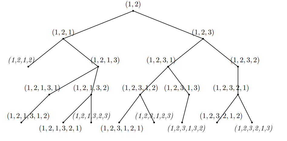
We give an illustration of the algorithm in Figure 4 for paths up to length \(6\) in \(Q_3.\) We have represented the algorithm as a rooted tree, with root \((1,2),\), i.e., our initial path in the algorithm. The paths of length \(3\) constructed from \((1,2)\) are shown by the branches of the root, and we continue so on till we get paths of length \(6.\) The paths shown in bold type are cycles.
We also prove that any two types of a path of length \(k\) obtained from the algorithm are different, i.e., there does not exist an automorphism between any two types.
Theorem 2.5. In a hypercube \(Q_n,~ n\geq 2,\) types of a path of length \(k\) obtained from the above algorithm are mutually distinct.
Proof. We prove the result by induction on \(k.\)
For \(k=2,\) we get path \((1,2)\) by the algorithm. But that is the only type of path of length \(2,\) by Lemma 2.4.
Suppose \(k=3.\) Then by the algorithm, we get two types (say) \(P_1=(1,2,1)\) and \(P_2=(1,2,3).\) Suppose there exists an automorphism \(\phi,\) such that \(\phi(P_1)=P_2.\) But then \(\phi(1)=1,\phi(2)=2\) and \(\phi(1)=3,\) which is a contradiction to \(\phi\) is one-to-one, being an automorphism. So the two types \(P_1\) and \(P_2\) are distinct.
Assume the result for types of path of length \(k-1.\)
Let \(P\) and \(Q\) be two types of path of length \(k\) generated by the algorithm. So suppose the type \(P\) is given by \((i_1,i_2,\ldots,i_{k-1},i_k).\) Then the sequence \((i_1,i_2,\ldots,i_{k-1})\) corresponds to the type (say) \(P'\) of path of length \(k-1,\) from which \(P\) is generated in the algorithm by adding a direction \(i_k.\) Similarly, let \(Q\) be given by \((j_1,j_2,\ldots,j_{k-1},j_k),\) such that \(Q'=(j_1,j_2,\ldots,j_{k-1})\) is the corresponding type of length \(k-1.\)
If \(P'=Q',\) then by construction in the algorithm, we must have \(i_k\neq j_k,\) as \(P\) and \(Q\) are not the same.
Suppose \(P'\neq Q',\) i.e., \(P'\) and \(Q'\) are two distinct types of path of length \(k-1,\) generated by the algorithm. Now suppose if possible, there exists an automorphism \(\phi\) such that \(\phi(P)=Q.\) But then one will get \(\phi(P')=Q',\) a contradiction to the induction hypothesis. Therefore there does not exist an automorphism between \(P\) and \(Q.\) ◻
We prove that, by using the algorithm, one gets all possible types of paths of length \(k,\) where \(2\leq k \leq 2^n.\)
Theorem 2.6. In a hypercube \(Q_n,\) \(n\geq 2,\) all the types of a path of length \(k,\) where \(2\leq k \leq 2^n,\) are generated by the above algorithm.
Proof. We prove the result by induction on \(k.\)
For \(k=2,\) the type \((1,2)\) is the initial path of the algorithm. But by Theorem 2.5, it is the only type for path of length \(2.\)
Suppose \(k=3.\) Then by the algorithm, we get two types (say) \(P_1=(1,2,1)\) and \(P_2=(1,2,3).\) We claim that these are the only two types of path of length \(3.\) Suppose if possible, there exists another type (say) \(Q=(i_1,i_2,i_3)\) of the path of length \(3.\) Then we have the following cases.
Case 1. If \(i_1=i_2=i_3,\) then \(Q\) is not a path of length \(3.\)
Case 2. Suppose any two among \(i_1,i_2,i_3\) are same and the third is different. Then in order to form a path of length \(3,\) the direction sequence must have equal directions at the first and third place. So we must have \(i_1=i_3.\) So \(Q=(i_1,i_2,i_1).\) But then there exists a permutation \(\phi=(1,i_1)(2,i_2)\) such that \(\phi(P_1)=Q,\) a contradiction.
Case 3. Suppose \(i_1,i_2,i_3\) are all distinct. Then there exists a permutation \(\phi=(1,i_1)(2,i_2)(3,i_3)\) such that \(\phi(P_2)=Q,\) a contradiction.
Therefore \(P_1\) and \(P_2\) are the only types of path of length \(3.\)
Assume the result for types of path of length \(k-1.\)
Now we prove the statement of the theorem for the types of path of length \(k.\) Suppose if possible there exists a type (say) \(P=(i_1,i_2,\ldots,i_{k-1},i_k)\) of path of length \(k,\) which is distinct from the types we get by the algorithm. But then the sequence \((i_1,i_2,\ldots,i_{k-1})\) corresponds to the type (say) \(P'\) of path of length \(k-1,\) from which \(P\) is generated, by adding a direction \(i_k.\) According to the induction hypothesis, all the types of path of length \(k-1\) are generated in the algorithm. So there must be an automorphism, which takes \(P'\) to some type \(Q'\) of path of length \(k-1,\) generated by the algorithm. For convenience, we can consider \(P'=Q'.\)
Now one needs to think about \(i_k.\) If \(i_k=i_j\) for some \(j\in\{1,2,k-1\},\) then \(i_k\) falls in the old set corresponding to \(P'\) in the algorithm. But then, in the algorithm, all the elements in the old set for \(P'\) are checked so as to get a valid type for path of length \(k\) from \(P'.\) So if \(P\) is a valid path type, then we are through. Suppose \(i_k\neq i_j,\) for all \(j=1,2,\ldots,k-1.\) Then \(i_k\) belongs to the new set corresponding to \(P'.\) In the algorithm, we consider only the smallest element from the new set corresponding to \(P'\) for constructing a path type of length \(1\) more than \(P'.\) Let \(s\) be the smallest element of the new set corresponding to \(P'.\) If \(i_k=s,\) we get \(P\) from the algorithm. If not, then there exists a permutation \(\theta=(i_k,s),\) such that \(\theta(P)\) is a type of path of length \(k\) generated by the algorithm. ◻
A path of length \(k\) in a hypercube needs at the most \(k\) directions, while a cycle of length \(k\) needs at the most \(k/2\) directions. So we have the following remark.
Remark 2.7. Suppose \(Q_k\) is a subcube of \(Q_n,\) i.e., \(k\leq n.\) Then the types of paths upto length \(k\) in \(Q_k\) are the only types of paths upto length \(k\) in \(Q_n.\) Similarly, the types of cycles upto length \(2k\) in \(Q_k\) are the only types of cycles upto length \(2k\) in \(Q_n.\)
We are particularly interested in the types of a \(k\)-cycle in hypercube \(Q_n,\) where \(k\) is even and \(4\leq k\leq 2^n.\) From the above algorithm, we get all types of cycles as well. In fact one can write a computer program to get all the types of a \(k\)-cycle in \(Q_n.\) We could generate all the types of \(k\)-cycles in \(Q_4\) using that program, where \(k\) is even and \(4\leq k \leq 16.\) In fact, for \(n=4\) itself, we got \(392\) types of cycles of length \(14.\) One needs a super computer to generate the paths and cycles of \(Q_n,\) even if \(n\) is as small as \(6.\)
In the next section, we discuss all possible cycle decompositions of \(Q_4.\)
Notation 3.1. We use ‘ \(\sqcup\) ’ for the union of edge disjoint graphs and ‘ \(\uplus\) ’ for the union of vertex disjoint graphs.
Note that \(|V(Q_4)|=2^4=16\) and \(|E(Q_4)|=32.\) We look at the problem of finding cycle decompositions of \(Q_4\) in view of partitioning the number \(32\) as \(k_1+k_2+\ldots+k_r,\) where \(k_i\)’s are all even and \(4\leq k_i \leq 16,~ i=1,2,\ldots,r.\) Following is the list of such partitions.
| 16+16 | 16+10+6 | 16+8+4+4 | 16+6+6+4 |
|---|---|---|---|
| 14+14+4 | 14+12+6 | 14+10+8 | 14+10+4+4 |
| 14+8+6+4 | 14+6+6+6 | 12+12+8 | 12+12+4+4 |
| 12+10+10 | 12+10+6+4 | 12+8+8+4 | 12+8+6+6 |
| 12+8+4+4+4 | 12+6+6+4+4 | 12+4+4+4+4+4 | 10+10+8+4 |
| 10+10+6+6 | 10+8+8+6 | 10+8+6+4+4 | 10+6+6+6+4 |
| 10+6+4+4+4+4 | 8+8+8+8 | 8+8+8+4+4 | 8+8+6+6+4 |
| 8+8+4+4+4+4 | 8+6+6+4+4+4 | 6+6+6+6+4+4 | 4+4+4+4+4+4+4+4 |
| 16+ 12+ 4 | 16+ 8+ 8 | 16+4+4+4+4 | 14+6+4+4+4 |
| 10+10+4+4+4 | 8+6+6+6+6 | 8+4+4+4+4+4+4 | 6+6+4+4+4+4+4 |
We observe that, there exists a cycle decomposition corresponding to the partitions with white background in Table 1. However, corresponding to the partitions with a pink background, there does not exist any cycle decomposition of \(Q_4,\) which we have verified with the help of the algorithm. In Table 2, possible cycle decompositions of \(Q_4\) are drawn.
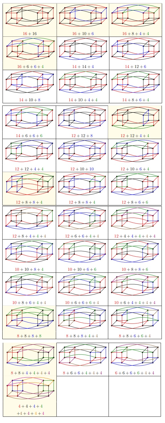
In the table, the \(2\)-regular, spanning subgraphs of \(Q_4\) are shown in the cells with yellow background. They are called as \(2\)-factors. From these factorizations of \(Q_4\) we can get factorizations of hypercubes of higher dimensions.
Now we discuss the cycle decomposition of \(Q_4\) with perfect matchings, which also leads to the cycle decompositions of higher dimensional cubes.
Graham and Harary [5] proved that there are \(272\) different perfect matchings of \(Q_4.\) In each of the above possible cycle decompositions, we can have many perfect matchings that can be selected from the cycles in the decomposition.
For illustration, consider the first Hamiltonian decomposition of \(Q_4\) in Table 2. We can choose different perfect matchings from the given cycle decomposition of \(Q_4\) as shown in Table 3.
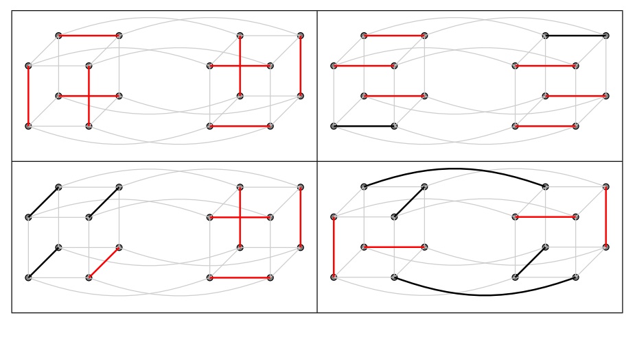
These decompositions will help us to get cycle decompositions of \(Q_6\) as given in the next section.
In this section, we find some cycle decompositions of \(Q_6, Q_8, \ldots.\)
Theorem 4.1 (Induction step for Hypercubes).Let \(n \geq 6\) be even. Suppose \(Q_{n-2}\) can be decomposed into \(r(n-2)\)-cycles \(C_1,C_2,\ldots,C_s\) where \(s = 2^{n-r-3}\) such that each \(C_i\) contains \(r\) edges \(e_{i1},e_{i2}, \ldots e_{ir},\) such that the set \(M_i=\{e_{ij} ~\colon~ j = 1,2,\ldots,r; ~ i = 1,2, \ldots, s\}\) forms a perfect matching in \(Q_{n-2}.\) Then \(Q_n\) can be decomposed into \(rn\)-cycles \(Z_1,Z_2,\ldots,Z_{4s}\) such that each \(Z_i\) contains \(r\) edges \(f_{i1},f_{i2}, \ldots f_{ir},\) such that the set \(\{f_{ij} ~\colon~ j = 1,2,\ldots,r; ~ i = 1,2, \ldots, 4s\}\) forms a perfect matching in \(Q_{n}.\)
Proof. Write \(Q_n\) as \(Q_n=Q_{n-2} \Box ~ Q_{2}.\) Let \(H=Q_{n-2},\) \(G=Q_n\) and \(Q_2\) is nothing but a \(4\)-cycle. Now \(Q_{n-2}\) is decomposed into \(r(n-2)\)-cycles, viz. \(C_1,C_2,\ldots,C_s.\) Further, from each \(C_i,\) a set of \(r\) edges, viz. \(M_i=\{e_{i1},e_{i2}, \ldots e_{ir}\}\) is selected such that \(\displaystyle \bigcup_{i=1}^s M_i\) forms a perfect matching in \(Q_{n-2}.\) So \(Q_n\) has a decomposition into cycles \(C_1^j,C_2^j,\ldots,C_s^j,\) \(j=1,2,3,4\) of length \(r(n-2)+2r=rn.\) Further, each \(C_i^j\) contains a set \(M_i^{j+1}\) of \(r\) edges such that \(\displaystyle\bigcup_{j=1}^{4}\bigcup_{i=1}^{s}M_i^j\) is a perfect matching of \(Q_n\) (addition for \(j\) is taken modulo \(4\).) Rename cycle \(C_i^j\) as \(Z_{(j-1)s+i}\) and edge \(e_{it}^{j+1}\in M_i^{j+1}\) as \(f_{js+i~t}\) where \(i=1,2,\ldots,s,\) \(t=1,2,\ldots,r\) and \(j=1,2,3,4.\) Hence the result. ◻
We give illustration of the theorem below.
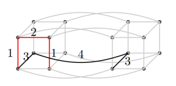
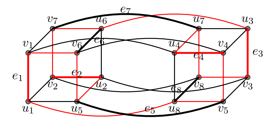
Illustration. Consider a hamiltonian decomposition of \(Q_4\) into cycles \(C_1\) (red colour) and \(C_2\) (black colour) along with a perfect matching containing \(4\) edges each from both the cycles (shown by bold edges in Figure 5). Let the edges from cycle \(C_1\) contributing to the perfect matching be \(\{e_1=(u_1,v_1),e_2=(u_2,v_2),e_3=(u_3,v_3),e_4=(u_4,v_4)\}\) and those from \(C_2\) be \(\{e_5=(u_5,v_5),e_6=(u_6,v_6),e_7=(u_7,v_7),e_8=(u_8,v_8)\}.\)
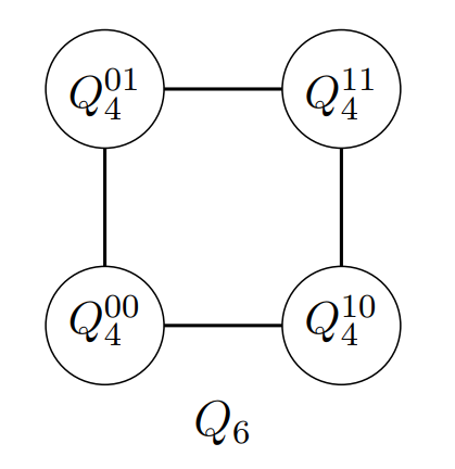
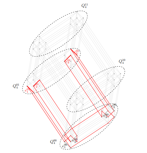
We construct \(24\)-cycles in \(Q_6\) from the \(16\)-cycles in the above decomposition and edges of perfect matching in \(Q_4.\) We know that \(Q_6=Q_4\Box Q_2,\) where \(Q_2\) is nothing but a \(4\)-cycle. So \(Q_6\) consists of four copies of \(Q_4\) (say) \(Q_4^{00}, Q_4^{01}, Q_4^{11}\) and \(Q_4^{10},\) whose corresponding vertices are joined as shown by connections given in the following Figure 6.
Let \(C_1^{ij}\) and \(C_2^{ij}\) be the \(16\)-cycles in \(Q_4^{ij}\) and let \(u_k^{ij},v_k^{ij}\) be the end vertices of the edges \(e_k^{ij}\) in the perfect matching of \(Q_4^{ij},\) \(i,j\in\{0,1\},\) \(k\in\{1,2,\ldots,8\}.\)
Now the \(24\)-cycles which decompose \(Q_6\) are as follows.
(a) \[\begin{aligned} Z_1=&[C_1^{00}~\setminus~\{e_1^{00},e_2^{00},e_3^{00},e_4^{00}\}] \cup \{e_1^{01},e_2^{01},e_3^{01},e_4^{01},(u_1^{00},u_1^{01}), (u_2^{00},u_2^{01}),(u_3^{00},u_3^{01}),\\ &(u_4^{00},u_4^{01}), (v_1^{00},v_1^{01}),(v_2^{00},u_2^{01}),(v_3^{00},v_3^{01}),(v_4^{00},v_4^{01})\} \end{aligned}\]
(b) \[\begin{aligned} Z_2=&[C_1^{01}\setminus\{e_1^{01},e_2^{01},e_3^{01},e_4^{01}\}] \cup \{e_1^{11},e_2^{11},e_3^{11},e_4^{11},(u_1^{01},u_1^{11}),(u_2^{01},u_2^{11}),(u_3^{01},u_3^{11}),\\&(u_4^{01},u_4^{11}),(v_1^{01},v_1^{11}),(v_2^{01},u_2^{11}),(v_3^{01},v_3^{11}),(v_4^{01},v_4^{11})\} \end{aligned}\]
(c) \[\begin{aligned} Z_3=&[C_1^{11}\setminus\{e_1^{11},e_2^{11},e_3^{11},e_4^{11}\}] \cup \{e_1^{10},e_2^{10},e_3^{10},e_4^{10},(u_1^{11},u_1^{10}),(u_2^{11},u_2^{10}),(u_3^{11},u_3^{10}),\\&(u_4^{11},u_4^{10}),(v_1^{11},v_1^{10}),(v_2^{11},u_2^{10}),(v_3^{11},v_3^{10}),(v_4^{11},v_4^{10})\} \end{aligned}\]
(d) \[\begin{aligned} Z_4=&[C_1^{10}\setminus\{e_1^{10},e_2^{10},e_3^{10},e_4^{10}\}] \cup \{e_1^{00},e_2^{00},e_3^{00},e_4^{00},(u_1^{10},u_1^{00}),(u_2^{10},u_2^{00}),(u_3^{10},u_3^{00}),\\&(u_4^{10},u_4^{00}), (v_1^{10},v_1^{00}),(v_2^{10},u_2^{00}),(v_3^{10},v_3^{00}),(v_4^{10},v_4^{00})\} \end{aligned}\]
(e) \[\begin{aligned} Z_5=&[C_2^{00}\setminus\{e_5^{00},e_6^{00},e_7^{00},e_8^{00}\}] \cup \{e_5^{01},e_6^{01},e_7^{01},e_8^{01},(u_5^{00},u_5^{01}),(u_6^{00},u_6^{01}),(u_7^{00},u_7^{01}),\\&(u_8^{00},u_8^{01}), (v_5^{00},v_5^{01}),(v_6^{00},u_6^{01}),(v_7^{00},v_7^{01}),(v_8^{00},v_8^{01})\} \end{aligned}\]
(f) \[\begin{aligned} Z_6=&[C_2^{01}\setminus\{e_5^{01},e_6^{01},e_7^{01},e_8^{01}\}] \cup \{e_5^{11},e_6^{11},e_7^{11},e_8^{11},(u_5^{01},u_5^{11}),(u_6^{01},u_6^{11}),(u_7^{01},u_7^{11}),\\&(u_8^{01},u_8^{11}),(v_5^{01},v_5^{11}),(v_6^{01},u_6^{11}),(v_7^{01},v_7^{11}),(v_8^{01},v_8^{11})\} \end{aligned}\]
(g) \[\begin{aligned} Z_7=&[C_2^{11}\setminus\{e_5^{11},e_6^{11},e_7^{11},e_8^{11}\}] \cup \{e_5^{10},e_6^{10},e_7^{10},e_8^{10},(u_5^{11},u_5^{10}),(u_6^{11},u_6^{10}),(u_7^{11},u_7^{10}),\\&(u_8^{11},u_8^{10}),(v_5^{11},v_5^{10}),(v_6^{11},u_6^{10}),(v_7^{11},v_7^{10}),(v_8^{11},v_8^{10})\} \end{aligned}\]
(h) \[\begin{aligned} Z_8=&[C_2^{10}\setminus\{e_5^{10},e_6^{10},e_7^{10},e_8^{10}\}] \cup \{e_5^{00},e_6^{00},e_7^{00},e_8^{00},(u_5^{10},u_5^{00}),(u_6^{10},u_6^{00}),(u_7^{10},u_7^{00}),\\&(u_8^{10},u_8^{00}),(v_5^{10},v_5^{00}),(v_6^{10},u_6^{00}),(v_7^{10},v_7^{00}),(v_8^{10},v_8^{00})\} \end{aligned}\]
See Figure 7 for better understanding where we have shown the construction of cycle \(Z_1.\) One can construct the remaining cycles in the decomposition on the similar lines.
Because cycles \(C_1\) and \(C_2\) of \(Q_4\) are edge disjoint, it can be easily verified that the cycles \(Z_1,Z_2,\ldots,Z_8\) are mutually edge disjoint. Moreover, all the cross edges between any two copies of \(Q_4\) are exhausted, as they are taken along the edges of perfect matching in \(Q_4.\) Therefore we get edge decomposition of \(Q_6\) into cycles of length \(24.\)
Moreover as \(Q_6\) contains four copies of \(Q_4\) and perfect matchings in all of them are selected. Then \(\displaystyle\bigcup_{i=1}^8 M_i\) gives a perfect matching in \(Q_6,\) where \(M_i\) is the set of edges from \(Z_i,\) contributing to a perfect matching of \(Q_6.\)
The following table gives the generalization of cycle decomposition of \(Q_4\) with a perfect matching to the corresponding cycle decomposition of \(Q_n,\) with a perfect matching.
| \(Q_4=C_1\cup C_2\) | Corresponding cycle | Corresponding cycle | Corresponding cycle | |
|---|---|---|---|---|
| 1-2 \(m_1\) | \(m_2\) | decomposition of \(Q_6\) | decomposition of \(Q_8\) | decomposition of \(Q_n\) |
| \(8\) | \(0\) | \(4 \times C_{32} + 4 \times C_{16}\) | \(16 \times C_{48} + 16 \times C_{16}\) | \(2^{n-4}\times C_{8(n-2)}+2^{n-4}\times C_{16}\) |
| \(6\) | \(2\) | \(4 \times C_{28} + 4 \times C_{20}\) | \(16 \times C_{40} + 16 \times C_{24}\) | \(2^{n-4}\times C_{6(n-2)+4}+2^{n-4}\times C_{2(n-4)+16}\) |
| \(5\) | \(3\) | \(4 \times C_{26} + 4 \times C_{22}\) | \(16 \times C_{36} + 16 \times C_{28}\) | \(2^{n-4}\times C_{5(n-2)+6}+2^{n-4}\times C_{3(n-4)+16}\) |
| \(4\) | \(4\) | \(8 \times C_{24}\) | \(32 \times C_{32}\) | \(2^{n-3} \times C_{4n}\) |
Theorem 4.2. Let \(n \geq 4\) be even. Then the hypercube \(Q_n\) can be decomposed into \(4n\)-cycles (say) \(C_1, C_2, \ldots, C_r,\) where \(r = 2^{n-3}\) such that
(I) every \(C_i\) contains \(4\) edges \(e_{i1}, e_{i2}, e_{i3}, e_{i4}\) such that \(C_i \setminus \{e_{i1}, e_{i2}, e_{i3}, e_{i4}\}\) has \(4\) components each of which is a path of length \(n-1\);
(II) \(M=\{e_{ij}~\colon~ j = 1, 2, 3, 4; i = 1, 2, \ldots, r\}\) forms a perfect matching in \(Q_n.\)
Proof. Proof of the theorem is by induction. For \(n=4\) and \(n=6,\) the result is true by Subsection 3.2 and illustration after Theorem 4.1 respectively. Proof of the induction step follows by Theorem 4.1. ◻
In this section, we discuss factorizations of \(Q_8\) obtained from those of \(Q_4,\) using properties of Cartesian product of graphs. We state a lemma, whose proof is trivial and follows from the definition of the Cartesian product of graphs.
Lemma 5.1. [11]
(a) Let a graph \(G_1\) be decomposed into spanning subgraphs \(H_1, H_2, \ldots, H_r\) and let a graph \(G_2\) be decomposed into spanning subgraphs \(F_1, F_2, \ldots,F_r.\) Then the graph \(G_1 \Box G_2\) can be decomposed into spanning subgraphs \(H_1 \Box F_1, H_2 \Box F_2, \ldots, H_r \Box F_r.\)
(b) Let \(G_1\) be a graph with components \(H_1, H_2, \ldots, H_r\) and let \(G_2\) be a graph with components \(F_1, F_2, \ldots, F_s.\) Then the components of \(G_1 \Box ~ G_2\) are \(H_i \Box ~ F_j\) with \(i= 1, 2, \ldots, r\) and \(j = 1, 2, \ldots, s.\)
We need the first part of the lemma for \(r=2.\) So we quote the following remark.
Remark 5.2. If graphs \(G_1\) and \(G_2\) are decomposed into two spanning subgraphs \(H_1, H_2\) and \(F_1, F_2\) respectively, then the graph \(G_1 \Box G_2\) can be decomposed into spanning subgraphs \(H_1 \Box F_1, H_2 \Box F_2.\) In fact, \(G_1 \Box G_2\) can be decomposed into spanning subgraphs \(H_1 \Box F_2\) and \(H_2 \Box F_1\) as well. So \(G_1\Box G_2\) has two decompositions \((H_1\Box F_1)\cup (H_2 \Box F_2)\) and \((H_1\Box F_2)\cup (H_2 \Box F_1).\)
We recall the following lemma by Kotzig.
Lemma 5.3([7]). Cartesian product of two cycles can be decomposed into two Hamiltonian cycles.
For the decomposition of \(Q_8\) using \(Q_4,\) we need \(2\)-factorizations of \(Q_4,\) i.e., decomposition of \(Q_4\) into \(2\)-regular, spanning subgraphs. Recall the table of all possible cycle decompositions of \(Q_4\) given in Section 3.1. In that table, we have coloured the cells having factorizations of \(Q_4.\) We call the two spanning subgraphs in each factorization of \(Q_4\) as \(H_1\) and \(H_2.\) Being \(2\)-regular, \(H_1,H_2\) consist of either a cycle or union of vertex disjoint cycles.
Now \(Q_8=Q_4 \Box Q_4.\) By Remark 5.2, corresponding to each pair of factorization \(H_1\sqcup H_2\) of \(Q_4,\) there exist two factorizations of \(Q_8,\) viz. \((H_1\Box H_1)\sqcup(H_2\Box H_2)\) and \((H_1\Box H_2)\sqcup(H_2\Box H_1).\) First, we give the Table 5 of factorizations of \(Q_4\) with reference from Table 2.
| Factorization of \(Q_4\) | \(H_1\) | \(H_2\) |
|---|---|---|
| \(C_{16} \sqcup C_{16}\) | \(C_{16}\) | \(C_{16}\) |
| \(C_{16} \sqcup (C_{10} \uplus C_6)\) | \(C_{16}\) | \(C_{10} \uplus C_6\) |
| \(C_{16} \sqcup (C_{8} \uplus C_4 \uplus C_4)\) | \(C_{16}\) | \(C_{8} \uplus C_4 \uplus C_4\) |
| \(C_{16} \sqcup (C_{6} \uplus C_6\uplus C_4)\) | \(C_{16}\) | \(C_{6} \uplus C_6\uplus C_4\) |
| \((C_{12}\uplus C_4) \sqcup (C_{12} \uplus C_4)\) | \(C_{12}\uplus C_4\) | \(C_{12}\uplus C_4\) |
| \((C_{12}\uplus C_4) \sqcup (C_{8} \uplus C_8)\) | \(C_{12}\uplus C_4\) | \(C_{8} \uplus C_8\) |
| \((C_{8} \uplus C_8)\sqcup (C_{8} \uplus C_8)\) | \(C_{8} \uplus C_8\) | \(C_{8} \uplus C_8\) |
| \((C_{8} \uplus C_{8} )\sqcup (C_4\uplus C_4\uplus C_4\uplus C_4)\) | \(C_{8} \uplus C_8\) | \(C_4\uplus C_4\uplus C_4\uplus C_4\) |
| \((C_4\uplus C_4\uplus C_4\uplus C_4)\sqcup (C_4\uplus C_4\uplus C_4\uplus C_4)\) | \(C_4\uplus C_4\uplus C_4\uplus C_4\) | \(C_4\uplus C_4\uplus C_4\uplus C_4\) |
Now we work out two factorizations of \(Q_8\) corresponding to one of the factorizations of \(Q_4.\)
We deliberately consider a factorization, where \(H_1\) and \(H_2\) are non-isomorphic.
Factorization of \(Q_4\): \(C_{16} \sqcup (C_{10} \uplus C_6)\)’
\[H_1=C_{16} \text{ and } H_2=(C_{10} \uplus C_6). \text{ So }Q_4=H_1\sqcup H_2.\]
Factorizations of \(Q_8\):
\[\begin{aligned} Q_8=&Q_4 \Box Q_4 = (H_1\sqcup H_2)\Box(H_1\sqcup H_2)\\ =&(H_1\Box H_1)\sqcup(H_2\Box H_2)\ldots (I)\\ =&(H_1\Box H_2)\sqcup(H_2\Box H_1)\ldots (II),\qquad\qquad\qquad(\text{by Remark 5.2}.) \end{aligned}\]
As \(H_1\neq H_2,\) here (I) and (II) will give two different factorizations of \(Q_8\) as follows.
(I). \[\begin{aligned} Q_8=&(H_1\Box H_1)\sqcup(H_2\Box H_2)\\ =&[C_{16}\Box C_{16}]\sqcup [(C_{10} \uplus C_6)\Box (C_{10} \uplus C_6)]\\ =&[C_{16}\Box C_{16}]\sqcup [(C_{10}\Box C_{10})\uplus(C_{10}\Box C_6)\uplus(C_{6}\Box C_{10})\uplus(C_{6}\Box C_6)],\qquad \text{(by Lemma 5.1(2).)} \end{aligned}\]
Now by Lemma 5.3, the Cartesian product of two cycles can be decomposed into two Hamiltonian cycles (say) \(C^1_{256}\) and \(C^2_{256}.\) So \(C_{16}\Box C_{16}=C^1_{256}\sqcup C^2_{256},\) where vertex set of the cycles \(C^1_{256}\) and \(C^2_{256}\) is the same. We get cycles from the other brackets on the similar lines. Therefore
\[Q_8=[C^1_{256}\sqcup C^2_{256}]\sqcup[(C^1_{100}\sqcup C^2_{100})\uplus(C^1_{60}\sqcup C^2_{60})\uplus(C^1_{60}\sqcup C^2_{60})\uplus (C^1_{36}\sqcup C^2_{36})].\]
So we get cycle decomposition of \(Q_8.\) In fact, we can regroup the cycles as follows to get the factorization of \(Q_8.\)
\[Q_8=C^1_{256}\sqcup C^2_{256}\sqcup [C^1_{100}\uplus C^1_{60}\uplus C^1_{60}\uplus C^1_{36}] \sqcup [C^2_{100}\uplus C^2_{60}\uplus C^2_{60}\uplus C^2_{36}].\]
(II). \[\begin{aligned} Q_8=&(H_1\Box H_2)\sqcup(H_2\Box H_1)=[C_{16}\Box (C_{10} \uplus C_6)]\sqcup [(C_{10} \uplus C_6)\Box C_{16}]\\ =&[(C_{16}\Box C_{10})\uplus(C_{16}\Box C_{6})]\sqcup [(C_{10}\Box C_{16})\uplus(C_{6}\Box C_{16})],\quad \text{(by Lemma 5.1(2).)} \end{aligned}\]
\[Q_8=[(C^1_{160}\sqcup C^2_{160})\uplus(C^1_{96}\sqcup C^2_{96})]\sqcup[(C^1_{160}\sqcup C^2_{160})\uplus(C^1_{96}\sqcup C^2_{96})],\quad \text{(by Lemma 5.3)}\]
\[Q_8=[C^1_{160}\uplus C^1_{96}]\sqcup [C^2_{160}\uplus C^2_{96}]\sqcup [C^1_{160}\uplus C^1_{96}] \sqcup [C^2_{160}\uplus C^2_{96}],\] is the factorization of \(Q_8.\)
Observe that the two factorizations of \(Q_8\), which we get from a single factorization of \(Q_4\) are non-isomorphic.
Remark 5.4. Consider the decomposition of \(Q_4\) into \(8\)-cycles. It is actually a factorization of \(Q_4.\) From this factorization, we get a factorization of \(Q_8\) into \(64\)-cycles. In fact, one can choose \(8\) edges from each cycle in this decomposition of \(Q_8,\) such that their union forms a perfect matching.
One can repeat the above procedure to get factorizations of \(Q_{16}\) from the factorizations of \(Q_8\) and so on to get factorizations of \(Q_n,\) where \(n\) is a power of \(2.\)
In this paper, we gave an algorithm and its complexity to find all possible types of paths in \(Q_n.\) In particular, from the types of cycles, we get a complete list of all possible and impossible cycle decompositions of \(Q_4.\) Using cycle decompositions of \(Q_4\) along with perfect matchings, various cycle decompositions of \(Q_6, Q_8\) and in general \(Q_n\) can also be obtained. Moreover, the factorization of \(Q_8\) using factorization of \(Q_4\) is obtained. One can generalise the process to get factorizations of \(Q_n\) for \(n\) power of \(2,\) from the factorizations of \(Q_{n/2}\).