
Semi-conductors, such as silicon, offer affordability, non-toxicity, and find widespread utility in electronics, being integral to the functioning of nearly all electronic devices. Silicon carbide (SiC), composed of lightweight elements, exhibits a low thermal expansion coefficient, strong covalent bonds, high thermal conductivity, and remarkable hardness. Discovered by the American scientist E.G. Acheson in 1891, this material was hailed as the hardest substance on Earth until 1929. SiC presents various colors, such as green or black, upon the adding of impurities like aluminum (Al), iron (Fe), or oxygen (O). Due to its exceptional heat resistance, SiC finds application in furnace components such as heating elements, core tubes, and refractory bricks. Moreover, it serves as a precursor for graphene sheets [1, 2]. Its versatile properties contribute to its extensive usage in electronics, transportation vehicles, and applications in quantum physics. For further insights, refer to [3, 4, 5]. This paper delves into the topological properties of silicon carbide \(SiC_{4}\)–\(I[r,s]\).
Chemical graph theory is a field of discrete mathematics that addresses various chemical challenges. It involves the exploration of chemical structures present in molecular compounds relevant to pharmaceuticals and artificial food products [5, 6, 7, 8, 9, 10]. The interdisciplinary nature of chemical graph theory lies in its connection between chemistry and mathematics. Notably, graph theory was pioneered by Euler in the 18th century [11].
In chemical graph theory, molecules are typically represented as simple connected graphs, with chemical bonds depicted as edges and atoms as vertices. This graphical representation enables scientists to investigate and comprehend isomerism phenomena in chemical compounds. By studying the graph structures, researchers can analyze the behavior of different isomers of the same chemical compound.
Furthermore, chemical graph theory finds applications in the detection and resolution of drug-related issues [12, 13, 14, 15].
The numerical value associated with a molecular graph is known as a topological index, which represents a unique type of graph invariant. These molecular descriptors play a significant role in Quantitative Structure-Activity Relationship (QSAR) studies [16]. A topological index can be conceptualized as a function that assigns each molecular structure a real number. One of the earliest topological indices introduced is the Wiener index, proposed by H. Wiener in 1947 [17].
Topological indices serve as valuable tools for predicting the physicochemical properties and bioactivity of chemical compounds. Over the years, hundreds of topological descriptors have been defined to better understand the structural characteristics of these compounds [18].
The concept of \(\nu\varepsilon\)–degree and \(\varepsilon\nu\)–degree based Topological Indices (TIs) in graph theory was proposed by Chellali et al. [19]. Subsequently, Horoldagva et al. [20] extended these indices to mathematics. The \(\nu\varepsilon\)–degree and \(\varepsilon\nu\)–degree based Zagreb and Randić indices are considered more powerful than classical vertex-type indices. For more detailed information about \(\varepsilon\nu\)–degree and \(\nu\varepsilon\)–degree based TIs, refer to [21, 22, 23]. Zhong [24] introduced the harmonic index, while Randić defined the Randić index in 1975 [25], and Gutman introduced the first and second Zagreb indices [26]. Initially, these indices were based on classical degrees, but the \(\epsilon\nu\)-degree and \(\nu\epsilon\)-degree versions of these TIs offer more benefits. For more advanced information about graphs, silicon carbide, \(\epsilon\nu\)-degree and \(\nu\epsilon\)-degree, and topological indices, see [27, 28, 29, 30, 31].
Let \(\zeta)= (V, E)\) be an undirected, connected, and simple graph, where \(E(\zeta)\) denotes the collection of edges and \(V(\zeta)\) denotes the collection of nodes. A simple graph is one that does not have a loop or multiple edges. If a graph has a connection between any two nodes, it is said to be connected. Silicon carbide’s 2D molecular structures are both simple and interconnected. The degree of a vertex \(\nu\), denoted as \(\text{deg}(\nu)\), is the number of vertices connected to a fixed vertex \(\nu\). An edge \(e\) is represented by \(e = \upsilon\omega \in E(\zeta)\).
If \(\zeta\) is a simple connected graph, the degree (\(\text{deg}(\upsilon)\)) represents the count of different edges incident to any node within the closed neighborhood of \(\upsilon\). The vertex-edge degree (\(\nu\varepsilon\text{-degree}\)) can be calculated by considering the number of distinct edges incident on any node \(\upsilon\) within its open neighborhood. Moreover, the edge-vertex degree (\(\varepsilon\nu\text{-degree}\)) of an edge \(\check{e}\) is defined as the count of vertex unions between the open neighborhoods of the endpoints \(\omega\) and \(\upsilon\). The \(\varepsilon\nu\text{-degree}\) and \(\nu\varepsilon\text{-degree}\) based Topological Indices (TIs) are presented below in mathematical notation.
The \(\varepsilon\nu\) degree-based Zagreb index can be determined as follows: \[M^{ev}(\zeta)=\sum\limits_{e\varepsilon E} deg_{ev}(e)^{2}.\] The 1\(^{st}\) \(\nu\varepsilon\)–degree Zagreb alpha index \((M^{\alpha ve}_{1}\)(\(\zeta\))) is determined as: \[M^{\alpha ve}_{1}(\zeta)=\sum\limits_{\upsilon\varepsilon V} deg_{ev}(\upsilon)^{2}.\] The 1\(^{st}\) \(\nu\varepsilon\)–degree Zagreb beta index \((M^{\beta ve}_{1}\)(\(\zeta\))) computed as: \[M^{\beta ve}_{1}(\zeta)=\sum\limits_{\upsilon\omega\varepsilon E} deg_{ve}(\omega)+ deg_{ve}(\upsilon).\] The second \(\nu\varepsilon\)–degree Zagreb index \((M^{ve}_{2}\)(\(\zeta\))) mathematically defined as: \[M^{ve}_{2}(\zeta)=\sum\limits_{\upsilon\omega\varepsilon E} (deg_{ve}(\omega)\times deg_{ve}(\upsilon)).\] The \(\nu\varepsilon\)–degree Randić index (R\(^{ve}\)(\(\zeta\))) mathematically satiated as: \[R^{ve}(\zeta)=\sum\limits_{\upsilon\omega\varepsilon E} (deg_{ve}(\omega)\times deg_{ve}(\upsilon))^{\frac{-1}{2}}.\] The \(\varepsilon\nu\)–degree Randić index (\(R^{ev}\)(\(\zeta\))) determined as: \[R^{ev}(\zeta)=\sum\limits_{e\varepsilon E} (deg_{ve}(e))^{\frac{-1}{2}}.\] The \(\nu\varepsilon\)–degree Atom Bond Connectivity index (ABC\(^{ve}\)(\(\zeta\))) calculated by formula given below, as: \[ABC^{ve}(\zeta)=\sum\limits_{\upsilon\omega\varepsilon E}\sqrt{\frac{deg_{ve}(\omega)+ deg_{ve}(\upsilon)-2}{deg_{ve}(\omega)\times deg_{ve}(\upsilon)}}.\] The \(\nu\varepsilon\)–degree Geometric Arithmetic index (GA\(^{ve}\)(\(\zeta\))) determined as: \[GA^{ve}(\zeta)=\sum\limits_{\omega\upsilon\varepsilon E}2\frac{\sqrt{deg_{ve}(\omega)\times deg_{ve}(\upsilon)}}{deg_{ve}(\omega)+ deg_{ve}(\upsilon)}.\] The \(\nu\varepsilon\)–degree Harmonic index (H\(^{ve}\)(\(\zeta\))): \[H^{ve}(\zeta)=\sum\limits_{\omega\upsilon\varepsilon E(G)}\frac{2}{deg_{ve}(\omega)+ deg_{ve}(\upsilon)}.\] The \(\nu\varepsilon\)–degree Sum-Connectivity index (X\(^{ve}\)(\(\zeta\))) computed as: \[X^{ve}(\zeta)=\sum\limits_{\omega\upsilon\varepsilon E(G)}(deg_{ve}(\omega)+ deg_{ve}(\upsilon))^{\frac{-1}{2}}.\] Yamac and Cancan discuss this \(\varepsilon\nu\) and \(\nu\varepsilon\) degree based TIs for the Sierpinski Gasket Fractal in 2009 [27].
We utilized a diverse array of methodologies to obtain our findings, encompassing the edge parcel technique, vertex segment strategy, graph hypothetical device, degree verification tactic, and combinatorial techniques. In this investigation, we applied various tools and methodologies. For computational tasks and verification processes, MATLAB was employed, while MAPLE was utilized for generating 2D and 3D graphs. Additionally, chem-sketch software was employed for constructing structural graphs of \(SiC_{4}-I[r,s]\).
The \(2D\) molecular graph of \(SiC_{4}\)–\(I[r,s]\) is shown in Figure \(1\). Any chemical compound’s building block is the unit cell, as we all know. A molecular structure is made up of a huge number of unit cells arranged in a certain pattern.In a molecular structure, r represents the number of unit cells in a row, where s represents the number of rows. In Figure \(1\) a unit cell and a structure of \(r=2\) and \(s=1\), \(r=3\) and \(s=2\) and \(r=s=3\) are represented. Consequently, the total numbers of vertices, edges and faces in \(SiC_{4}-I[r,s]\) are; \[\begin{aligned} |V(SiC_4-I[r,s])|&=10rs,\\ |E(SiC_4-I[r,s])|&=12rs-r-s,\\ |F(SiC_4-I[r,s])|&=2rs-r-s+2. \end{aligned}\]
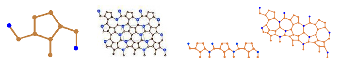
The unit cell is used to compute silicon carbide formulae \(SiC_{4}\)–\(I[r,s]\). To raise \(r\), interconnect the unit cells horizontally, then connect the rows vertically to increase \(s\). The connection points must be correct. Where \(r\) is the number of rows and \(s\) is the number of columns.
There are \(3\) kinds of nodes based on the degree of nodes. Vertices of 1\(_{st}\), 2\(^{nd}\) and 3\(_{rd}\) degree are represented as \(V_{1}\), \(V_{2}\) and \(V_{3}\) respectively as shown in Table 1.
| \([r,s]\) | \([1,1]\) | \([2,1]\) | \([3,1]\) | \([1,2]\) | \([2,2]\) | \([3,2]\) | \([1,3]\) | \([2,3]\) | \([3,3]\) |
|---|---|---|---|---|---|---|---|---|---|
| \(V_{1}\) | 3 | 6 | 9 | 3 | 6 | 9 | 3 | 6 | 9 |
| \(V_{2}\) | 4 | 6 | 8 | 8 | 10 | 12 | 12 | 14 | 16 |
| \(V_{3}\) | 3 | 8 | 13 | 9 | 24 | 39 | 15 | 40 | 65 |
| deg(\(\omega\)) | Cardinality |
|---|---|
| \(V_{1}\) | \(3r\) |
| \(V_{2}\) | \(2r+4s-2\) |
| \(V_{3}\) | \(10rs-5r-4s+2\) |
| Total vertices | Total edges |
|---|---|
| \(10rs\) | \(15rs-4r-2s+1\) |
By using above methodology we will partition the edges of \(SiC_{4}\)–\(I[r,s]\). In the instance of \(SiC_{4}\)–\(I[r,s]\), there are five distinct edge portions, as shown in Table 4. It is important to note that the variables \(r,s\geq1\).
| \((\text{deg}(\omega),\text{deg}(\upsilon))\) | \(\varepsilon\nu\)–degree | Cardinality |
|---|---|---|
| \((2,1)\) | \(3\) | \(2\) |
| \((3,1)\) | \(4\) | \(3r-2\) |
| \((2,2)\) | \(4\) | \(r+2s-2\) |
| \((3,2)\) | \(5\) | \(2r+4s-2\) |
| \((3,3)\) | \(6\) | \(15rs-10r-8s+5\) |
In this section, we calculate the main results for silicon carbide \(SiC_{4}\)–\(I[r,s]\). We calculate the TIs using different basic definitions and values given in tables. The specific TI index uses specific values in the table and provides information about the correlation coefficient. These correlation constants represent the connection between the numerical number and the characterization of any graph or network.
| \(deg(\omega)\) | \(\upsilon\varepsilon\)–degree | Cardinality |
|---|---|---|
| 1 | 2 | 2 |
| 1 | 3 | \(2r-2\) |
| 2 | 4 | 2 |
| 2 | 5 | \(2r+4s-4\) |
| 3 | 6 | 2 |
| 3 | 7 | \(3r\) |
| 3 | 8 | \(2r+4s-6\) |
| 3 | 9 | \(10rs-10r-8s+8\) |
| deg(\(\omega\)),deg(\(\upsilon\)) | \(\varepsilon\nu\)–degree | Cardinality |
|---|---|---|
| (3,1) | (7,3) | \(3r-2\) |
| (2,1) | (4,2) | 2 |
| (2,2) | (5,5) | \(r+2s-2\) |
| (2,2) | (7,4) | 1 |
| (3,2) | (7,5) | 3 |
| (3,2) | (8,4) | 1 |
| (3,2) | (8,5) | \(2r+4s-7\) |
| (3,3) | (8,7) | \(r+1\) |
| (3,3) | (8,8) | \(s-1\) |
| (3,3) | (9,7) | \(5r-3\) |
| (3,3) | (9,8) | \(3r+6s-11\) |
| (3,3) | (9,9) | \(15rs-19r-15s+19\) |
By making use of \(\varepsilon\nu\)–degree of edge partitions of \(SiC_{4}\)–\(I[r,s]\), as shown in Table 5, we calculate the \(M^{ev}\) index in the following lines: \[\begin{aligned} M^{ev}(SiC_{4}-I[r,s]) &= \sum\limits_{e \in E(SiC_{4}-I[r,s])}(deg_{ev}(e)^{2}) \\ &= 2 \times 3^{2} + (3r-2) \times 4^{2} + (r+2s-2) \times 4^{2} \\ &\quad+ (2r+4s-2) \times 5^{2} + (15rs-10r-8s+5) \times 6^{2} \\ &= 540rs-246r-156s+84. \end{aligned}\]
By making use of \(\nu\varepsilon\)–degree of vertices partition of \(SiC_{4}\)–\(I[r,s]\) for \(r,s\geq2\), as seen in Table 5, we compute the \(M^{\alpha ve}_{1}\) in the following lines: \[\begin{aligned} M^{\alpha ve}_{1}(SiC_{4}-I[r,s]) &= \sum\limits_{\upsilon \in V(SiC_{4}-I[r,s])}(deg_{ve}(\upsilon)^{2}) \\ &= 2 \times 2^{2} + (3r-2) \times 3^{2} + 2 \times 4^{2} \\ &\quad+ (2r+4s-4) \times 5^{2} + (3r) \times 7^{2} \\ &\quad+ (2r+4s-6) \times 8^{2} + (10rs-10r-8s+8) \times 9^{2} \\ &= 810rs-458r-292s+186. \end{aligned}\]
By making use of \(\nu\varepsilon\)–degree based partition of the end vertices of the edges of \(SiC_{4}\)–\(I[r,s]\) for \(r,s\geq2\), as shown in Table 6, we compute the \(M^{\beta ve}_{1}\) in the following lines: \[\begin{aligned} M^{\beta ve}_{1}(SiC_{4}-I[r,s]) &= \sum\limits_{\omega\upsilon \in E(SiC_{4}-I[r,s])}(deg_{ve}(\omega) + deg_{ve}(\upsilon)) \\ &= (3r-2) \times 10 + 6 \times 2 + (r+2s-2) \times 10 + 1 \times 11 \\ &\quad+ 3 \times 12 + (2r+4s-7) \times 13 + 1 \times 12 \\ &\quad+ (5r-3) \times 16 + (3r+6s-11) \times 17 \\ &\quad+ (r+1) \times 15 + (s-1) \times 16 + (15rs-19r-15s+19) \times 18 \\ &= 270rs-130r-80s+46. \end{aligned}\]
Simply availing use of \(\nu\varepsilon\)–degree based partition of end vertices of the edges of \(SiC_{4}\)–\(I[r,s]\) for \(r,s\geq2\), using Table 6, we compute the \(M^{ve}_{2}\) in the following lines: \[\begin{aligned} M^{ve}_{2}(SiC_{4}-I[r,s]) &= \sum\limits_{\omega\upsilon \in E(SiC_{4}-I[r,s])}( deg_{ve}(\omega) \times deg_{ve}(\upsilon)) \\ &= (3s-2) \times 21 + 2 \times 8 + (r+2s-2) \times 25 + 1 \times 28 \\ &\quad+ 3 \times 35 + (2r+4s-7) \times 40 + 1 \times 32 \\ &\quad+ (5r-3) \times 63 + (3r+6s-11) \times 72 \\ &\quad+ (r+1) \times 56 + (s-1) \times 64 + (15rs-19r-15s+19) \times 81 \\ &= 1215rs-784r-509s+359. \end{aligned}\]
By utilizing the \(\nu\varepsilon\)–degree based partition of end vertices of the edges of \(SiC_{4}\)–\(I[r,s]\) for \(r,s\geq2\), as given in Table 6, we compute the \(R^{ve}\) as follows, \[\begin{aligned} R^{ve}(SiC_{4}-I[r,s]) &= \sum\limits_{\omega\upsilon \in E(SiC_{4}-I[r,s])}(deg_{ve}(\omega)\times deg_{ve}(\upsilon))^{\frac{-1}{2}} \\ &= (3r-2)\times(21)^{\frac{-1}{2}}+2\times(8)^{\frac{-1}{2}}+(r+2s-2)\times(25)^{\frac{-1}{2}} \\ &\quad+ 1\times(28)^{\frac{-1}{2}}+3\times(35)^{\frac{-1}{2}}+(2r+4s-7)\times(40)^{\frac{-1}{2}}+1 \\ &\quad\times(32)^{\frac{-1}{2}}+(5r-3)\times(63)^{\frac{-1}{2}}+(3r+6s-11)\times(72)^{\frac{-1}{2}} \\ &\quad+(r+1)\times(56)^{\frac{-1}{2}}+(s-1)\times(64)^{\frac{-1}{2}}+(15rs-19r-15s+19)\times(81)^{\frac{-1}{2}} \\ &= \frac{5}{3}rs+\left(\frac{3}{\sqrt{21}}+\frac{1}{\sqrt{10}}+\frac{5}{3\sqrt{7}}+\frac{1}{2\sqrt{2}}+\frac{1}{2\sqrt{14}}-\frac{86}{45}\right)r \\ &\quad+\left(\frac{2}{\sqrt{10}}+\frac{1}{\sqrt{2}}-\frac{137}{120}\right)s \\ &\quad+\left(\frac{-2}{\sqrt{21}}-\frac{1}{2\sqrt{7}}+\frac{1}{\sqrt{2}}+\frac{3}{\sqrt{35}}-\frac{7}{2\sqrt{10}}+\frac{1}{4\sqrt{2}}\right.\\ &\quad\left.+\frac{13}{12\sqrt{2}}-\frac{11}{6\sqrt{2}}+\frac{1}{2\sqrt{14}}+\frac{571}{360}\right) \\ &=1.66rs+0.176r+0.197s+0.082. \end{aligned}\]
By utilizing the \(\varepsilon\nu\)–degree of edges partition of \(SiC_{4}\)–\(I[r,s]\) for \(r,s\geq2\), as given in Table 5, we compute the \(R^{ev}\) as follows, \[\begin{aligned} R^{ev}(SiC_{4}-I[r,s]) &= \sum \limits_{e \in E(SiC_{4}-I[r,s])}(deg_{ve}(e)^{\frac{-1}{2}}) \\ &= 2\times(3)^{\frac{-1}{2}}+(3r-2)\times(4)^{\frac{-1}{2}}+(r+2s-2)\times(4)^{\frac{-1}{2}} \\ &\quad +(2r+4s-2)\times(5)^{\frac{-1}{2}}+(15rs-10r-8s+5)\times(6)^{\frac{-1}{2}} \\ &= \frac{15}{\sqrt{6}}rs+\left(\frac{2}{\sqrt{5}}-\frac{10}{\sqrt{6}}+2\right)r+\left(\frac{4}{\sqrt{5}}-\frac{8}{\sqrt{6}}+1\right)s \\ &\quad+\left(\frac{2}{\sqrt{3}}-\frac{2}{\sqrt{5}}+\frac{5}{\sqrt{6}}-2\right) \\ &=6.12rs-1.18r-0.47s+0.3015. \end{aligned}\]
With the help of \(\nu\varepsilon\)–degree based partition of the end vertices of the edges of \(SiC_{4}\)–\(I[r,s]\) for \(r,s\geq2\), as shown in Table 6, we compute the \(ABC^{ve}\) as follows, \[\begin{aligned} ABC^{ve}(SiC_{4}-I[r,s]) &= \sum\limits_{\omega\upsilon \in E(SiC_{4}-I[r,s])}\sqrt{\frac{deg_{ve}(\omega)+deg_{ve}(\upsilon)-2}{deg_{ve}(\omega)\times deg_{ve}(\upsilon)}}\\ &= (3r-2)\times\sqrt{\frac{8}{21}}+2\times\sqrt{\frac{84}{8}}+(r+2s-2)\times\sqrt{\frac{8}{25}}+1\times\sqrt{\frac{9}{28}} \\ &\quad +3\times\sqrt{\frac{10}{35}}+(2r+4s-7)\times\sqrt{\frac{11}{40}}+\sqrt{\frac{10}{32}} \\ &\quad+(5r-3)\times\sqrt{\frac{14}{63}}+(3r+6s-11)\times\sqrt{\frac{15}{72}} \\ &\quad+(r+1)\times\sqrt{\frac{13}{56}}+(s-1)\times\sqrt{\frac{14}{64}}+(15rs-19r-15s+19)\times\sqrt{\frac{16}{81}}\\ &=\frac{20}{3}rs+\left(6\frac{\sqrt{2}}{21}+2\frac{\sqrt{2}}{5}+4\frac{\sqrt{11}}{\sqrt{10}}+5\frac{\sqrt{2}}{3}+\frac{3\sqrt{5}}{2\sqrt{6}}\right.\\ &\quad+\left.\frac{1\sqrt{13}}{2\sqrt{7}}-\frac{76}{9}\right)r+\left(4\frac{\sqrt{2}}{5}+8\frac{\sqrt{11}}{\sqrt{10}}+3\frac{\sqrt{5}}{\sqrt{6}}+\frac{\sqrt{14}}{\sqrt{8}}-\frac{20}{3}\right)s \\ &\quad+\left(\frac{2}{\sqrt{2}}-4\sqrt{\frac{2}{21}}-4\frac{\sqrt{2}}{5}+\frac{3}{2\sqrt{7}}+3\sqrt{\frac{2}{5}}\right.\\ &\quad\left.-14\frac{\sqrt{11}}{\sqrt{10}}+\frac{\sqrt{5}}{4}-\sqrt{2}+\frac{1\sqrt{5}}{2\sqrt{6}}+\frac{1\sqrt{14}}{2\sqrt{7}}-\frac{\sqrt{14}}{8}+\frac{76}{9}\right)\\ & =667rs+257r+6.06s-4.911. \end{aligned}\]
By making use of \(\nu\varepsilon\)–degree based partition of the end vertices of the edges of \(SiC_{4}\)–\(I[r,s]\) for \(r,s\geq2\), as shown in Table 6, we compute the \(GA^{ve}\) as follows, \[\begin{aligned} GA^{ve}(SiC_{4}-I[r,s]) &= \sum_{\omega\upsilon \in E(SiC_{4}-I[r,s])}(2\frac{\sqrt{\deg_{ve}(\omega)\times\deg_{ve}(\upsilon)}}{\deg_{ve}(\omega)+\deg_{ve}(\upsilon)}) \\ &= (3r-2)\times2\frac{\sqrt{21}}{10}+4\frac{\sqrt{8}}{6}+(r+2s-2)\times2\frac{\sqrt{25}}{10}+2\times\frac{\sqrt{28}}{11}\\ &\quad +6\times\frac{\sqrt{35}}{12}+(2r+4s-7)\times2\frac{\sqrt{40}}{13}+2\frac{\sqrt{32}}{12}+(5r-3)\times2\frac{\sqrt{63}}{16}\\ &\quad +(3r+6s-11)\times2\frac{\sqrt{72}}{17}+(r+1)\times2\frac{\sqrt{56}}{15}+(s-1)\times2\frac{\sqrt{64}}{16}\\ &\quad +(15rs-19r-15s+19)\times2\frac{\sqrt{81}}{18}\\ &=15rs+\left(3\frac{\sqrt{21}}{5}+8\frac{\sqrt{10}}{13}+15\frac{\sqrt{7}}{8}+36\frac{\sqrt{2}}{17}+4\frac{\sqrt{14}}{15}-18\right)r\\ &\quad+\left(16\frac{\sqrt{10}}{13}+72\frac{\sqrt{2}}{17}-2\right)s+\left(4\frac{\sqrt{2}}{3}-2\frac{\sqrt{21}}{5}+4\frac{\sqrt{7}}{11}\right.\\ &\quad\left.+4\frac{\sqrt{7}}{11}+\frac{\sqrt{35}}{2}-28\frac{\sqrt{10}}{3}+2\frac{\sqrt{2}}{3}+\frac{9\sqrt{7}}{8}\right.\\ &\quad\left.-132\frac{\sqrt{2}}{17}+4\frac{\sqrt{14}}{13}+16\right)\\ &=15rs-4.35r+7.88s+8.213. \end{aligned}\]
By making use of \(\nu\varepsilon\)–degree based partition of the end vertices of the edges of \(SiC_{4}\)–\(I[r,s]\) for \(r,s\geq2\), as shown in Table 6, we compute the \(H^{ve}\) as follows, \[\begin{aligned} H^{ve}(SiC_{4}-I[r,s]) &= \sum\limits_{\omega\upsilon \in E(SiC_{4}-I[r,s])} \frac{2}{deg_{ve}(\omega)+ deg_{ve}(\upsilon)}\\ &= 2\times\frac{(3r-2)}{10}+\times\frac{4}{6}+2\times\frac{(r+2s-2)}{10}+\frac{2}{11}+\frac{6}{12}+2\times\frac{(2r+4s-7)}{13}\\ &\quad+\frac{2}{12}+2\times\frac{(5r-3)}{16}+2\times\frac{(3r-6s-11)}{17}+2\times\frac{(r+1)}{15}+2\times\frac{(s-1)}{16}\\ &=\frac{5}{3}rs+\frac{8581}{79560}r+\frac{5263}{26520}s-\frac{1472}{1989}\\ &=1.667rs+0.107r+0.198s+0.74. \end{aligned}\]
By making use of \(\nu\varepsilon\)–degree based partition of the end vertices of the edges of \(SiC_{4}\)–\(I[r,s]\) for \(r,s\geq2\), as shown in Table 6, we compute the \(X^{ve}\) as follows, \[\begin{aligned} X^{ve}(SiC_{4}-I[r,s]) &= \sum_{\omega\upsilon\in E(SiC_{4}-I[r,s])}(deg_{ve}(\omega)+ deg_{ve}(\upsilon))^{\frac{-1}{2}} \\ &= \frac{3r-2}{\sqrt{10}} + \frac{2}{\sqrt{6}} + \frac{r+2s-2}{\sqrt{10}} + \frac{1}{\sqrt{11}} + \frac{3}{\sqrt{12}} + \frac{2r+4s-7}{\sqrt{13}} \\ &\quad+ \frac{1}{\sqrt{12}} + \frac{3r-3}{\sqrt{16}} + \frac{3r+6s-11}{\sqrt{17}} + \frac{r+1}{\sqrt{15}} + \frac{s-1}{\sqrt{16}} \\ &\quad+ \frac{15rs-19r-15s+19}{\sqrt{18}} \\ &= \frac{5}{\sqrt{2}}rs + \left(\frac{5}{\sqrt{10}}+\frac{3}{\sqrt{17}}+\frac{1}{\sqrt{15}}-\frac{19}{3\sqrt{2}}+\frac{5}{3}\right)r \\ &\quad+ \left(\frac{6}{\sqrt{10}}+\frac{6}{\sqrt{17}}-\frac{5}{\sqrt{2}}+\frac{1}{4}\right)s + \left(\frac{2}{\sqrt{6}}-\frac{11}{\sqrt{10}}+\frac{1}{\sqrt{11}} \right. \\ &\quad\left.+\frac{2}{\sqrt{3}}-\frac{11}{\sqrt{17}}+\frac{1}{\sqrt{15}}+\frac{19}{3\sqrt{2}}-1\right) \\ &= 3.53rs – 0.244r + 0.067s – 0.137. \end{aligned}\]
The topological indices provide an easy way to convert chemical composition into numerical values that can be correlated with physical characteristics in QSPR research. The ev and ve-related indices give more effective results as compared to classical indices in various cases. For instance, the correlation coefficient between the acentric factor of 18 isomers of octane and the classical first Zagreb index is moderate (\(r = -0.7889\)), but the ev-degree Zagreb index shows excellent values of correlation as \(R = – 0.9808\). Similarly, the correlation between properties of octane (acentric factor, boiling point, and entropy) and classical R-index is very low, as \(r(AF) = 0.4048\)4, \(r(S) = 0.3506\), and \(r(BP) = 0.0737\), but ev-degree-related Randić indices give amazing values of coefficients like \(R(AF) = 0.8475\), \(R(S) = 0.8441\), and \(R(BP) = 0.7807\). The H-index also shows moderate correlation values with the characteristics of 18 isomers of octane: r(AF) = 0.7998, r(entropy) = 0.7594, and r(BP) = 0.801. This ev-degree type approach is also effective in discussing the structural features of the alkane family and SiC isomers.
Application of silicone carbide in physical perspective, deoxidizer used in steel making, one of the most widely used refractory materials with the best economic benefits, high-quality abrasive for sandblasting. Furthermore, because of small amounts of iron or different contaminating influences from the current generation, this is typically discovered as a somewhat blue dark, brilliant crystalline strong. In this study, we defined topological invariants of silicon carbide \(SiC_{4}\)–\(I[r,s]\) based on \(\varepsilon\nu\)–degree and \(\nu\varepsilon\)–degree. The findings are extremely valuable and beneficial from both a chemical and pharmacological standpoint. In future, we can find \(\varepsilon\nu\)–degree and \(\nu\varepsilon\)–degree topological indices of some nanostar dendrimers.
The authors declare no conflict of interest.
Malkesh Singh is receiving funds from SMVDU vide Grant/Award Number: SMVDU/R&D/21/5121-5125 for this research.