
A subset \({\cal I}\) of vertices of a graph \(G\) is independent if no two vertices in \({\cal I}\) are adjacent in \(G\). The cardinality of a largest independent set of \(G\) is denoted by \(\alpha(G)\) and is called the vertex independence number of \(G\).
A subset \({\cal D}\) of the vertices of a graph \(G\) is dominating if every vertex \(v\) of \(G\) is an element of \({\cal D}\) or is adjacent in \(G\) to an element of \({\cal D}\). A dominating set \({\cal D}\) of \(G\) is minimal if no proper subset of \({\cal D}\) is a dominating set in \(G\). The cardinality of a largest minimal dominating set of \(G\) is denoted by \(\Gamma(G)\) and is called the upper domination number of \(G\).
The closed neighbourhood of a graph vertex \(v\), denoted by \(N[v]\), is the subset of all vertices of \(G\) that are adjacent to \(v\) in \(G\), together with the vertex \(v\) itself. The closed neighbourhood of a set of vertices \({\cal S}=\{v_1,\ldots,v_m\}\) of \(G\), denoted by \(N[{\cal S}]\), is simply \(N[{\cal S}]=\cup_{i=1}^{m}N[v_i]\). The set of private neighbours of a vertex \(v\in {\cal V}_G\) with respect to some subset \({\cal S}\subset {\cal V}_G\) is defined as \({\rm PN}(v,{\cal S})=N[v]\backslash N[{\cal S}\backslash\{v\}]\). A subset \({\cal X}\) of the vertices of \(G\) is irredundant if every vertex \(v\in {\cal X}\) has at least one private neighbour in \(G\) with respect to \({\cal X}\) (that is, if \({\rm PN}(v,{\cal X})\neq\emptyset\) for all \(v\in{\cal X}\)). Finally, the cardinality of a largest irredundant set of \(G\) is denoted by \(I\!R(G)\) and is called the irredundance number of \(G\).
It holds for any graph \(G\) that \[\alpha(G)\leq \Gamma(G) \leq I\!R(G),\label{domchain}\tag{1}\] a result dating back to 1978 that is due to Cockayne et al. [1].
A bi-colouring of the edges of a graph, using the colours red and blue, is called a red-blue edge colouring of the graph. If \(R\) and \(B\) are the subgraphs induced by respectively the red and the blue edges of such a colouring, the colouring is denoted by the ordered pair \((R,B)\), and \(R\) is referred to as the red subgraph, while \(B\) is called the blue subgraph.
The following six classes of Ramsey numbers have previously been defined in terms of the graph theoretic notions of independence, irredundance and domination.
The independent Ramsey number \(r=r(m,n)\) is the smallest natural number \(r\) such that in any red-blue edge colouring \((R,B)\) of the complete graph \(K_r\) of order \(r\), it holds that \(\alpha(B)\geq m\) or \(\alpha(R)\geq n\) (or both). This definition dates from 1930 and is due to Ramsey [2].
The irredundant Ramsey number \(s=s(m,n)\) is the smallest natural number \(s\) such that in any red-blue edge colouring \((R,B)\) of the complete graph \(K_s\) of order \(s\), it holds that \(I\!R(B)\geq m\) or \(I\!R(R)\geq n\) (or both). This definition dates from 1989 and is due to Brewster et al. [3].
The mixed irredundant Ramsey number \(t=t(m,n)\) is the smallest natural number \(t\) such that in any red-blue edge colouring \((R,B)\) of the complete graph \(K_t\) of order \(t\), it holds that \(I\!R(B)\geq m\) or \(\alpha(R)\geq n\) (or both). This definition dates from 1990 and is due to Cockayne et al. [4].
The upper domination Ramsey number \(u=u(m,n)\) is the smallest natural number \(u\) such that in any red-blue edge colouring \((R,B)\) of the complete graph \(K_u\) of order \(u\), it holds that \(\Gamma(B)\geq m\) or \(\Gamma(R)\geq n\) (or both). This definition dates from the early 1990s and is due to Oellermann and Shreve [5].
The mixed domination Ramsey number \(v=v(m,n)\) is the smallest natural number \(v\) such that in any red-blue edge colouring \((R,B)\) of the complete graph \(K_v\) of order \(v\), it holds that \(\Gamma(B)\geq m\) or \(\alpha(R)\geq n\) (or both). This definition also dates from the early 1990s and is due to Oellermann and Shreve [5].
The irredundant-domination Ramsey number \(w=w(m,n)\) is the smallest natural number \(w\) such that in any red-blue edge colouring \((R,B)\) of the complete graph \(K_w\) of order \(w\), it holds that \(I\!R(B)\geq m\) or \(\Gamma(R)\geq n\) (or both). This definition dates from 2013 is due to Burger and Van Vuuren [6].
The arguments of the independent, irredundant and upper domination Ramsey numbers may be interchanged without altering the values of these numbers, i.e. \(r(m,n)=r(n,m)\), \(s(m,n)=s(n,m)\) and \(u(m,n)=u(n,m)\) for any integers \(m,n\geq 2\). In the case of the mixed Ramsey numbers \(t(m,n)\), \(v(m,n)\) and \(w(m,n)\), however, the arguments \(m\) and \(n\) do not necessarily commute, i.e., \(t(m,n)\neq t(n,m)\), \(v(m,n)\neq v(n,m)\) and \(w(m,n)\neq w(n,m)\) in general. Furthermore, these Ramsey numbers are related to each other by the inequality chains \[s(m,n) \leq w(m,n) \leq \left\{\begin{array}{c} u(m,n) \\ t(m,n)\end{array}\right\} \leq v(m,n) \leq r(m,n),\label{otherthansubgraphchains}\tag{2}\] which are easily shown to hold for all \(m,n\geq 2\) in view of (1). It is unknown in what way (if any) the Ramsey numbers \(u(m,n)\) and \(t(m,n)\) are related.
Apart from the infinite classes of Ramsey numbers \(x(2,n)=x(n,2)=n\) for all \(x\in\{r,s,t,u,v,w\}\) and all \(n\geq 2\), only 45 members of the above-mentioned six classes of Ramsey numbers are known exactly. These numbers are shown in Table 1. Our aim in this paper is to determine the two Ramsey numbers \(s(3,8)\) and \(w(3,8)\).
| \(s(m,n)\) | \(w(m,n)\) | \(u(m,n)\) | \(t(m,n)\) | \(v(m,n)\) | \(r(m,n)\) |
|---|---|---|---|---|---|
| \(s(3,3)=6^a\) | \(w(3,3)=6^b\) | \(u(3,3)=6^c\) | \(t(3,3)=6^d\) | \(v(3,3)=6^e\) | \(r(3,3)=6^f\) |
| \(s(3,4)=8^a\) | \(w(3,4)=8^b\) | \(u(3,4)=8^c\) | \(t(3,4)=9^d\) | \(v(3,4)=9^e\) | \(r(3,4)=9^f\) |
| \(s(3,5)=12^a\) | \(w(4,3)=8^b\) | \(u(3,5)=12^c\) | \(t(4,3)=8^d\) | \(v(4,3)=8^b\) | \(r(3,5)=14^f\) |
| \(s(3,6)=15^g\) | \(w(3,5)=12^b\) | \(u(3,6)=15^c\) | \(t(3,5)=12^d\) | \(v(3,5)=12^e\) | \(r(3,6)=18^i\) |
| \(s(3,7)=18^j\) | \(w(5,3)=12^b\) | \(u(4,4)=13^c\) | \(t(5,4)=13^d\) | \(v(5,3)=13^d\) | \(r(3,7)=23^{\ell}\) |
| \(\bf s(3,8)=21\) | \(w(3,6)=15^b\) | \(t(3,6)=15^h\) | \(v(3,6)=15^e\) | \(r(3,8)=28^m\) | |
| \(s(4,4)=13^k\) | \(w(6,3)=15^b\) | \(t(6,3)=15^b\) | \(v(6,3)=15^b\) | \(r(3,9)=36^n\) | |
| \(w(3,7)=18^o\) | \(t(3,7)=18^o\) | \(v(4,4)=14^b\) | \(r(4,4)=18^f\) | ||
| \(\bf w(3,8)=21\) | \(t(3,8)=22^o\) | \(r(4,5)=25^p\) | |||
| \(w(4,4)=13^b\) | \(t(4,4)=14^b\) |
Ramsey problems are known to be difficult, and it is accepted that the use of computers is inevitable when solving these problems. Considering all possible edge colourings works for smaller Ramsey problems, but in larger cases a more judicious approach is required. The algorithmic approach put forward in this paper for solving Ramsey problems of medium size offers a technique not seen before, which can be applied more widely than previous search tree approaches. It attempts to uncover a red-blue graph colouring systematically by looking for edges that necessarily have to be either red or blue graph, all the while making use of a set of rules/lemmas. It branches only into different cases when it can find no edges that are forced to be one colour or the other at that point during the search, and it eliminates cases that lead to contradictions. The chain of algorithmic deductions can, in fact, be printed by the algorithm in the format of a human-readable proof. This proof (by computer) can be shortened by using more sophisticated rules/lemmas. For this paper we chose to keep the number of rules limited and the nature of the rules themselves simple so as to avoid long and technical arguments. The algorithm is, however, generic in nature, in the sense that it can easily incorporate additional, newly established rules. A significant advantage of this approach is that the proof produced by the algorithm can be checked by another algorithm in a much shorter time than would be required to generate the proof in the first place.
The paper is organised as follows. After reviewing a number of preliminary results in §2, we present a recursive enumeration algorithm in §3 for determining bounds on any of the six types of Ramsey numbers mentioned above. In §4, we then show how the algorithm may be applied to determine the values of the two Ramsey numbers \(s(3,8)\) and \(w(3,8)\). The numerical results returned by the algorithm are presented and analysed in §5, after which the paper closes with suggestions for further work in §6.
Let \(x\in\{r,s,t,u,v,w\}\) be a Ramsey number. An \(x(m,n,p)\) colouring is a red-blue edge colouring \((R,B)\) of the complete graph \(K_p\) of order \(p\) which satisfies neither of the two sought-after chromatic conditions of the Ramsey number \(x(m,n)\), hence showing that \(x(m,n)>p\).
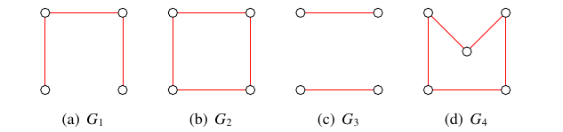
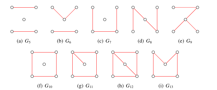
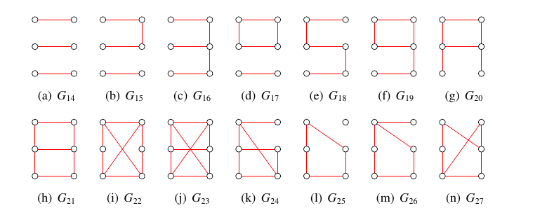
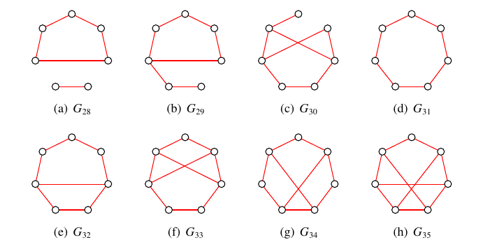
In [6], we computed complete sets of \(x(3,n,p)\) and \(x(m,3,p)\) colourings for all \(x\in\{s,t,u,v,w\}\), all \(m,n\in\{3,4,5,6\}\) and all admissible values of \(p\). In that paper, we also computed complete sets of \(x(4,4,p)\) colourings for all \(x\in\{s,t,u,v,w\}\) and all admissible values of \(p\). The red subgraphs of the complete sets of \(t(3,3,p)\) colourings of orders \(p=4\) and \(p=5\) are, for example, shown in Figure 1. The red subgraphs of the complete sets of \(t(3,4,p)\) colourings of orders \(5\), \(6\), \(7\) and \(8\) are similarly shown in Figures 2, 3, 4 and 5, respectively.
The following characterisation dates from 1989 and is due to Brewster et al. [3].
Lemma 1 ([3]). The blue subgraph of a red-blue edge colouring of a complete graph has an irredundant set of cardinality \(3\) if and only if there is a \(3\)-cycle in the red subgraph or a \(6\)-cycle \(v_1v_2v_3v_4v_5v_6v_1\) in the red subgraph with the edges \(v_1v_4\), \(v_2v_5\) and \(v_3v_6\) in the blue subgraph.
We call the second substructure in the above lemma a red \(6\)-cycle with blue diagonals. The following result relates \(x(m,n,p)\) colourings and \(y(m,n,p)\) colourings for different types \(x,y\in\{r,s,t,u,v,w\}\) of Ramsey numbers.
Lemma 2 ([6]). Let \(m,n>2\) be integers, and let \(x(m,n)\) and \(y(m,n)\) be two Ramsey numbers in (2) satisfying \(x(m,n)\leq y(m,n)\). Then any \(x(m,n,p)\) colouring is also a \(y(m,n,p)\) colouring.
The minimum degree of the subgraph \(R\) [\(B\), resp.] in a \(x(m,n,p)\) colouring \((R,B)\) is referred to as the minimum red [blue, resp.] degree and is denoted by \(\delta(R)\) [\(\delta(B)\), resp.]. Similar definitions hold for the maximum degrees of \(R\) and \(B\), denoted by \(\Delta(R)\) and \(\Delta(B)\), respectively.
Lemma 3 ([20]). Let \(m,n>2\) be integers. Then, \(\Delta(R)<s(m-1,n)\) and \(\Delta(B)<s(m,n-1)\) in any \(s(m,n,p)\) colouring \((R,B)\).
The following corollary follows from Lemma 3.
Corollary 1. Let \(m,n\geq 2\) be integers and let \(x\in\{r,s,t,u,v,w\}\) be a Ramsey number. Then, \(\Delta(R)<x(m-1,n)\) and \(\Delta(B)<x(m,n-1)\) in any \(x(m,n,p)\) colouring \((R,B)\).
Finally, the following useful result immediately follows from Corollary 1.
Corollary 2. Let \(m,n\geq 2\) be integers and let \(x\in\{r,s,t,u,v,w\}\) be a Ramsey number. Then, \(\delta(R)\geq p-x(m,n-1)\) and \(\delta(B)\geq p-x(m-1,n)\) in any \(x(m,n,p)\) colouring \((R,B)\).
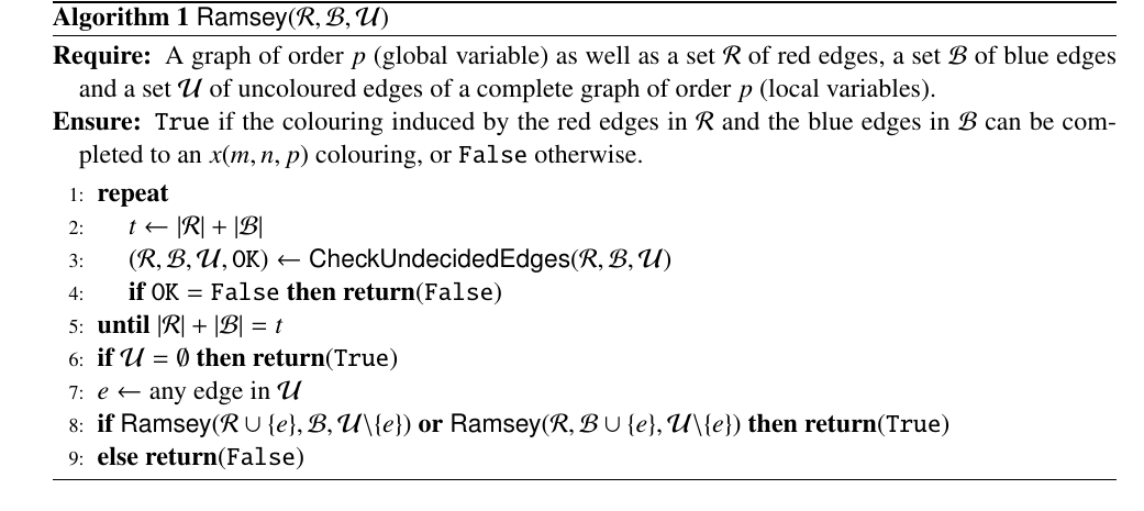
We present a recursive algorithm for deciding whether or not a partial red-blue edge colouring of a complete graph of order \(p\) can be completed to form an \(x(m,n,p)\) colouring, where \(x\in\{r,s,t,u,v,w\}\) is a Ramsey number. A pseudo-code listing of the algorithm is presented as Algorithm 1.
The algorithm takes as global input parameter a natural number \(p\) and as local input variables a set
\({\cal R}\) of red edges, a set \({\cal B}\) of blue edges and a set \({\cal U}\) of uncoloured edges of a
complete graph of order \(p\) and
essentially follows a branch-and-bound approach to yield the boolean
variable output True if the edges in \({\cal U}\) can be coloured red or blue in
some combination to form an \(x(m,n,p)\) colouring, or
False otherwise.
The external function \({\sf
CheckUndecidedEdges}({\cal R},{\cal B},{\cal U})\) is repeatedly
called (step 3) during the repeat-until loop (steps 1–5). This function
examines each edge in \({\cal U}\) in
turn, determining whether perhaps it must necessarily be coloured either
red or blue in order to avoid violating a so-called bounding
list of properties of an \(x(m,n,p)\) colouring. An example of such a
list of properties in the context of the Ramsey number \(r(3,4)\) is the bounding list in Table 2. If a colouring of any edge \(e\in{\cal U}\) is thus necessitated, the
edge \(e\) is removed from \({\cal U}\) and inserted into \({\cal R}\) or \({\cal B}\) (whichever is appropriate). In
addition to this set update, the function \({\sf CheckUndecidedEdges}({\cal R},{\cal B},{\cal
U})\) also updates the value of a global boolean variable
OK, originally initialised as having the value
True, to the value \({\tt False}\) if it is determined that some
edge \(e^*\in{\cal U}\) can be coloured
neither red nor blue (as a result of avoiding the contradiction of some
pair of properties in the bounding list). This process of calling the
function \({\sf CheckUndecidedEdges}({\cal
R},{\cal B},{\cal U})\) is repeated until the colouring of no
further edges in \({\cal U}\) is
necessitated by the bounding list.
| Property | Description |
|---|---|
| a | No red triangle is formed |
| b | No blue clique of order \(4\) is formed |
| c | The red degree of each vertex is at most \(3\) by Corollary 1 |
| d | The blue degree of each vertex is at most \(5\) by Corollary 1 |
If all edges have either been coloured red or blue (\({\cal U}=\emptyset\) in step 6), a valid
\(x(m,n,p)\) colouring has been found,
in which case the boolean value True is
returned. Otherwise, an edge \(e\in{\cal
U}\) is randomly selected (step 7) and branched upon, attempting
to colour it either red or blue by calling the algorithm recursively
with the updated input variable triples \({\cal R}\cup\{e\},{\cal B},{\cal
U}\backslash\{e\}\) or \({\cal R},{\cal
B}\cup\{e\},{\cal U}\backslash\{e\}\) (step 8). If this cannot be
achieved, then the boolean value False is
returned (step 9).
For some value \(p\) and a fixed
vertex \(v\in V(K_p)\), the set \({\cal R}\) may be initialised without loss
of generality in the context of seeking an \(x(m,n,p)\) colouring by taking \(p-x(m,n-1)\) arbitrary edges incident to
\(v\) according to Corollary 2. The set \({\cal B}\) may similarly be initialised by
taking any \(p-x(m-1,n)\) of the
remaining edges incident to \(v\). This
is illustrated in Figure 6(a) for \(v=1\) in the context of an \(r(3,4,8)\) colouring, upon which Algorithm
1 returns the boolean
value True, resulting in the \(r(3,4,8)\) colouring shown in Figure 6(b), which shows that
\(r(3,4)>8\).
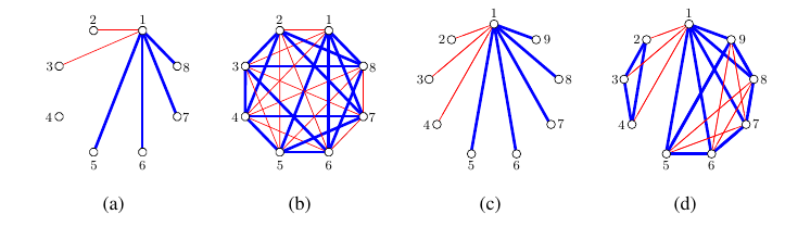
If, however, the same initialisation process is followed in the
context of an \(r(3,4,9)\) colouring,
as shown in Figure 6(c), Algorithm 1 returns the boolean
value False as a result of not being able to
compute an \(r(3,4,9)\) colouring,
because \(r(3,4)=9\). Although a
conceptually simple algorithm, the ranges of possible values of the
smallest unknown Ramsey numbers are currently so large that direct
application of Algorithm 1 to determine these
Ramsey numbers is not technologically possible. The rapid growth in the
number of branches and associated computing times required to determine
the Ramsey numbers \(r(3,n)\) for \(n\in\{3,4,5,6\}\) via Algorithm 1 is, for example,
illustrated in Table 3.
| Ramsey | Best lower bound | Best upper bound | ||||
|---|---|---|---|---|---|---|
| number | Value | Branches | Time | Value | Branches | Time |
| \(r(3,3)\) | \(>5\) | 2 | \(\ll 1\) | \(\leq 6\) | 0 | \(\ll 1\) |
| \(r(3,4)\) | \(>8\) | 12 | \(\ll 1\) | \(\leq 9\) | 234 | \(<1\) |
| \(r(3,5)\) | \(>13\) | 1 034 | \(<1\) | \(\leq 14\) | 0 | \(\ll 1\) |
| \(r(3,6)\) | \(>17\) | 7 969 625 | 276 | \(\leq 18\) | 6 944 615 486 | 416 233 |
There is, however, a better way of initialising the input sets \({\cal R}\) and \({\cal B}\) to Algorithm 1 than the initialisations shown in Figure 6 (a) and (c). Knowledge about smaller avoidance colourings may be utilised in the initialisations. The subgraph induced in any eventual \(r(3,4,9)\) colouring by the vertex subset \(\{5,6,7,8,9\}\) in Figure 6(c), for example, is necessarily an \(r(3,3,5)\) colouring, for if this were not the case, then the subgraph induced in the \(r(3,4,9)\) colouring by the vertex subset \(\{1,5,6,7,8,9\}\) would contain either a red triangle or a clique of order \(4\) as subgraph, a contradiction. Similarly, the subgraph induced in any eventual \(r(3,4,9)\) colouring by the vertex subset \(\{2,3,4\}\) in Figure 6(c) is necessarily an \(r(2,4,3)\) colouring, for otherwise the subgraph induced in the \(r(3,4,9)\) colouring by the vertex subset \(\{1,2,3,4\}\) would contain a red triangle as subgraph, again a contradiction. The input sets \({\cal R}\) and \({\cal B}\) to Algorithm 1 may therefore be initialised, without loss of generality, as shown in Figure 6(d), because there is only one \(r(2,4,3)\) colouring (a blue triangle) and only one \(r(3,3,5)\) colouring (consisting of a red five-cycle embedded within a blue five-cycle, as shown in Figure 1(d)).
When initialising the input sets \({\cal R}\) and \({\cal B}\) to Algorithm 1 as shown in Figure 6(d), the branching process illustrated in Figure 7 results, which shows that \(r(3,4)\leq 9\). In the figure, branching nodes are denoted by circles (containing the edges that are branched upon in coordinate form), while bounding nodes are denoted by rectangles (containing the reasons for contradictions preventing further growth of the tree in the form \(i\),\(j\)!xy which means that the edge \(ij\) can be coloured neither red because of reason x in Table 2 nor blue because of reason y in Table 2). Square brackets are used to present lists of edges whose colours are fixed by a branching decision, where a string of the form \(i\),\(j\)Rx means that the edge \(ij\) is necessarily red so as to avoid contradicting property x in Table 2, and similarly for blue edges. Angular brackets are used at the top of the tree to present a list of edge colours corresponding to the initialisation of the input sets \({\cal R}\) and \({\cal B}\) to Algorithm 1, where \(i\),\(j\)B means that edge \(ij\) is coloured blue, and similarly for red edges.
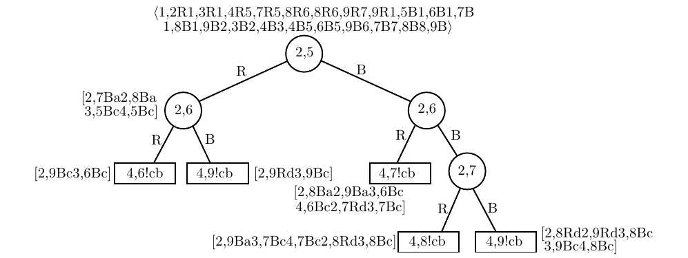
Note that because of the extended initialisation in Figure 6(d), the tree in Figure 7 has merely eight branches instead of the \(234\) branches that result according to Table 3 when the sparser initialisation in Figure 6(c) is used. But even with the denser initialisation procedure described above, which utilises information about smaller avoidance colourings, the rapid growth in the number of branches and associated computing times required by Algorithm 1 places the computation of most Ramsey numbers of the form \(r(3,n)\) for \(n>6\) out of the current reach of computing technology. It is, nevertheless, possible to apply the algorithm judiciously in order to determine some of these Ramsey number values, as we show in the next sections.
We denote the subgraph of the blue [red, resp.] subgraph of a \(t(m,n,p)\)-colouring induced by some set \(A\subseteq V(K_p)\) by \(\langle A\rangle_{{\rm blue}}\) [\(\langle A\rangle_{{\rm red}}\), resp.]. Let \(D_i(v)\) [\(D_{>i}(v)\) or \(D_{\geq i}(v)\), resp.] be the set of vertices at distance \(i\in\mathbb{N}\) [at a distance greater than \(i\) or at a distance at least \(i\), resp.] from some specified vertex \(v\) in the red subgraph of a \(t(3,n,p)\)-colouring. Since we avoid an irredundant set of cardinality \(3\) in the blue subgraph, we have the following useful result, adapted from [20].
Lemma 4 ([20]). Let \(v\) be any vertex of a \(t(3,n,p)\)-colouring.
If \(xyz\) is a path in \(\langle D_{>1}(v)\rangle_{{\rm red}}\) and \(x,z\in D_2(v)\), then \(x\) and \(z\) are joined by red edges to a common vertex in \(D_1(v)\).
If \(A\subseteq D_{>1}(v)\) contains at most one vertex of \(D_{>2}(v)\), then \(\langle A\rangle_{{\rm red}}\) is bipartite.
The following generalisation of the result in Lemma 4(a) is useful.
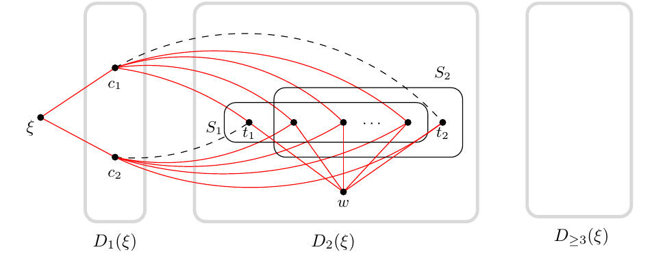
Corollary 3. Let \(K_{1,k}\) be a star in \(\langle D_{\geq 2}(\xi)\rangle_{{\rm red}}\) with centre in \(D_{\geq 2}(\xi)\) and endpoints in \(D_2(\xi)\). Then all the endpoints of this star have a common neighbour in \(D_1(\xi)\).
Proof. By induction on the number of endpoints of the star. The result of Lemma 4(a) serves as the base case for the induction. Suppose, as induction hypothesis, that all the endpoints in \(D_2(\xi)\) of any red star \(K_{1,k}\) with centre in \(D_{\geq 2}(\xi)\) have a common neighbour in \(D_1(\xi)\). We show by contradiction that all the endpoints in \(D_2(\xi)\) of any red star \(K_{1,k+1}\) with centre in \(D_{\geq 2}(\xi)\) have a common neighbour in \(D_1(\xi)\). Let \(S\) be the set of endpoints of such a star with centre \(w\), and let \(t_1\) and \(t_2\) be two vertices in \(S\). Suppose, to the contrary, that this star does not have a common neighbour in \(D_1(\xi)\). Let \(S_1\) and \(S_2\) be subsets of cardinality \(k\) of \(S\) such that \(S=S_1\cup\{t_2\}=S_2\cup\{t_1\}\), as shown in Figure 8. Then it follows by the induction hypothesis that all vertices in \(S_1\) have a common neighbour in \(D_1(\xi)\), and similarly for the vertices in \(S_2\). Let these common neighbours be \(c_1\) and \(c_2\), respectively. Then the edges \(c_1t_2\) and \(c_2t_1\) must both be blue (since the vertices in \(S\) do not all have a common neighbour in \(D_1(\xi)\)). But then \(\xi c_1t_1wt_2c_2\xi\) is a red six-cycle with blue diagonals \(\xi w\), \(c_1t_2\) and \(c_2t_1\) — contradicting Lemma 1. ◻
It follows from [18, Figure 4.1] that \(t(3,8,21)\) colourings exist. These colourings have, however, not yet been enumerated. Let \(\Xi\) and \(\overline{\Xi}\) be respectively the red and blue subgraphs of a \(t(3,8,21)\) colouring, and denote the minimum and maximum degrees of \(\Xi\) by \(\delta(\Xi)\) and \(\Delta(\Xi)\), respectively. Suppose \(\xi\) is a vertex of red degree \(\Delta(\Xi)\) in this colouring. Then the colourings in Figures 2–5 are relevant in the context of the \(t(3,8,21)\) colouring \((\Xi,\overline{\Xi})\) as a result of the following observation.
Observation 1. The colouring induced in \((\Xi,\overline{\Xi})\) by the vertices in \(D_{\geq 3}(\xi)\) is a \(t(3,8-\Delta(\Xi),20-|D_1(\xi)\cup D_2(\xi)|)\) colouring.
The subgraph \(\Xi\) also has the following properties.
Lemma 5 ([18, Lemmas 5–6)]. \(D_1(\xi)\) is an independent set of \(\Xi\), \(\Delta(\Xi)\leq 5\), \(|D_2(\xi)|\leq 11\) and \(|D_{>2}(\xi)|< t(3,8-\Delta(\Xi))\).
By Corollary 2, we therefore have the bounds \(3\leq \delta(\Xi) \leq \Delta(\Xi)\leq 5\). Note, however, that \(\Delta(\Xi)\neq 3\), for otherwise we would have a cubic graph \(\Xi\) of odd order. Therefore, \[4\leq \Delta(\Xi)\leq 5. \label{maxdegreebounds}\tag{3}\] The subgraph \(\langle D_2(\xi)\rangle_{{\rm red}}\) of \(\Xi\) is bipartite by Lemma 4(b). Suppose \(\langle D_2(\xi)\rangle_{{\rm red}}\) contains \(c\) components and denote the bipartitions of these components by \((X_i,Y_i)\) for all \(i=1,\ldots,c\). We call a component of the form \((X_i,Y_i)\) an \((|X_i|,|Y_i|)\) component, and we assume, without loss of generality, that \(|X_i|\geq |Y_i|\) for all \(i=1,\ldots,c\). Define \(X=\cup_{i=1}^{c}X_i\) and \(Y=\cup_{i=1}^{c}Y_i\). Then \(|X|\geq|Y|\).
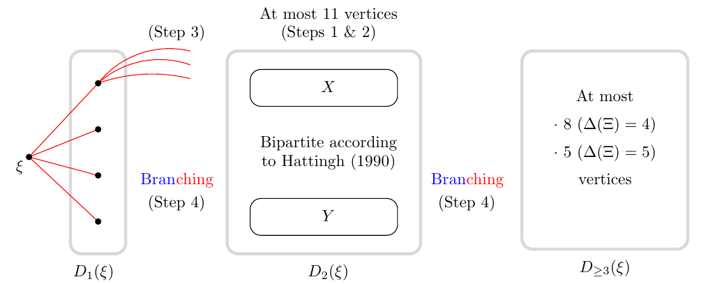
Our approach toward enumerating \(t(3,8,21)\) colourings consists of the following four steps:
| Subcase | \(|D_0(\xi)|\) | \(|D_1(\xi)|\) | \(|D_2(\xi)|\) | \(|X|\) | \(|Y|\) | \(|D_{>2}(\xi)|\) | Reference |
|---|---|---|---|---|---|---|---|
| I | 1 | 4 | 11 | 6 | 5 | 5 | [21, Table 7] |
| IIa | 1 | 4 | 10 | 6 | 4 | 6 | [21, Table 8] |
| IIb | 1 | 4 | 10 | 5 | 5 | 6 | [21, Table 9] |
| IIIa | 1 | 4 | 9 | 6 | 3 | 7 | [21, Table 10] |
| IIIb | 1 | 4 | 9 | 5 | 4 | 7 | [21, Table 11] |
| IVa | 1 | 4 | 8 | 6 | 2 | 8 | [21, Table 12] |
| IVb | 1 | 4 | 8 | 5 | 3 | 8 | Table 7 |
| IVc | 1 | 4 | 8 | 4 | 4 | 8 | [21, Table 14] |
| V | 1 | 5 | 11 | 6 | 5 | 4 | [21, Table 15] |
| VIa | 1 | 5 | 10 | 6 | 4 | 5 | [21, Table 16] |
| VIb | 1 | 5 | 10 | 5 | 5 | 5 | [21, Table 17] |
| Property | Description |
|---|---|
| e | No red triangle is formed; see Lemma 1 |
| f | No red \(6\)-cycle with blue diagonals is formed; see Lemma 1 |
| g | The red degree of each vertex is at most \(\Delta(\Xi)\); see (3) |
| h | Every vertex in \(D_2(\xi)\) is joined by a red edge to some vertex in \(D_1(\xi)\) |
| Property | Description |
|---|---|
| i | No red triangle is formed; see Lemma 1 |
| j | No red \(6\)-cycle with blue diagonals is formed; see Lemma 1 |
| k | The red degree of each vertex is at most \(\Delta(\Xi)\); see (3) |
| l | The endpoints in \(D_2(\xi)\) of a star in \(\langle D_{\geq 2}(\xi)\rangle_{{\rm red}}\) with centre in \(D_{\geq 2}(\xi)\) |
| all have a common neighbour in \(D_1(v)\); see Corollary 3 | |
| m | No odd red cycle is formed; see Lemma 4(b) |
| n | No blue complete graph of order \(7\) is formed in \(D_{\geq 2}(\xi)\) |
It is possible to rule out certain types of components in \(\langle D_{2}(\xi)\rangle_{{\rm red}}\). We start, however, by noting that in order to avoid a clique of order \(8\) in \(\langle \{\xi\}\cup X\cup D_{>3}(\xi)\rangle_{{\rm blue}}\), the following result holds.
Observation 2. If \(|X|=6\), then \(D_{>3}(\xi)=\emptyset\).
We also have the following restriction on small components of \(\langle D_{2}(\xi)\rangle_{{\rm red}}\).
Lemma 6. If \(|X|=6\), \(|Y|=5\) and \(\langle D_{2}(\xi)\rangle_{{\rm red}}\) has exactly one \((1,0)\) component, then \(\langle D_{2}(\xi)\rangle_{{\rm red}}\) is not a subgraph of \(\Xi\).
Proof. By contradiction. Suppose, to the contrary, that \(|X|=6\) and that \(\langle D_{2}(\xi)\rangle_{{\rm red}}\) has exactly one \((1,0)\) component in \(\Xi\). Then any vertex \(v\in D_3(\xi)\) is joined to the \((1,0)\) component by a red edge, for otherwise \(\langle \{\xi,v\}\cup D_{2}(\xi)\rangle_{{\rm blue}}\) contains a clique of order \(8\). The subgraph \(\langle D_3(\xi)\rangle_{{\rm red}}\) is therefore edgeless (so as to avoid triangles in \(\langle D_{\geq 2}(\xi)\rangle_{{\rm red}}\)). But then \(\langle D_{1}(\xi)\cup D_{3}(\xi)\rangle_{{\rm blue}}\) contains a clique of order \(9\) (and hence of order \(8\)), a contradiction. ◻
We similarly have the following restriction on large components of \(\langle D_{2}(\xi)\rangle_{{\rm red}}\).
Lemma 7. \(\langle D_{2}(\xi)\rangle_{{\rm red}}\) is not a \((6,5)\) component.
Proof. By contradiction. Suppose, to the contrary, that \(\langle D_{2}(\xi)\rangle_{{\rm red}}\) is a \((6,5)\) component. Since \(|X|=6\), it follows from Observation 2 that \(D_{>3}(\xi)=\emptyset\). Every vertex \(v\in D_3(\xi)\) is therefore joined to \(X\) by a red edge, for otherwise \(\langle\{\xi,v\}\cup X\rangle_{{\rm blue}}\) contains a clique of order \(8\). Hence all edges from \(D_3(\xi)\) to \(Y\) in \((\Xi,\overline{\Xi})\) are blue (so as to avoid odd cycles in \(\langle D_{\geq 2}(\xi)\rangle_{{\rm red}}\)). But then \(\langle \{\xi,v,w\}\cup Y\rangle_{{\rm blue}}\) contains a clique of order \(8\), by Lemma 4(b), since there is at least one blue edge \(vw\) for some pair \(v,w\in D_3(\xi)\), a contradiction. ◻
Suppose \(\Delta(\Xi)=4\). Then \(|D_2(\xi)|\leq 11\) and \(|D_{>2}(\xi)|<t(3,4)=9\) by Lemma 5. Furthermore, \(\langle D_{>1}(\xi)\rangle_{{\rm red}}\) does not contain a \((4,1)\) component (because of the red degree restriction on each vertex).
| No | X | Y | \(|\Phi_{\leq 2}|\) | \(|\Phi_{\geq 3}|\) | \(|\Phi|\) | Time |
|---|---|---|---|---|---|---|
| (i) | 1 1 3 | 0 0 3 | 14 | 2 | 0 | 143.3 |
| (ii) | 1 1 2 1 | 0 0 2 1 | 18 | 2 | 0 | 659.4 |
| (iii) | 1 1 1 1 1 | 0 0 1 1 1 | 10 | 2 | 0 | 212.2 |
| (iv) | 1 2 2 | 0 1 2 | 12 | 2 | 0 | 1 405.7 |
| (v) | 1 2 1 1 | 0 1 1 1 | 15 | 2 | 0 | 317.5 |
| (vi) | 1 3 1 | 0 2 1 | 19 | 2 | 0 | 84.1 |
| (vii) | 1 4 | 0 3 | 3 | 2 | 0 | 1.6 |
| (viii) | 2 2 1 | 1 1 1 | 9 | 2 | 3 | 274.3 |
| (ix) | 2 3 | 1 2 | 8 | 2 | 1 | 43.0 |
| (x) | 3 2 | 1 2 | 4 | 2 | 0 | 10.4 |
| (xi) | 3 1 1 | 1 1 1 | 2 | 2 | 0 | 7.7 |
| (xii) | 4 1 | 2 1 | 3 | 2 | 0 | 1.7 |
| (xiii) | 5 | 3 | 0 | — | 0 | 0.1 |
The results obtained when applying our four-step enumeration process described above to subcases I–IVc in Table 4 are presented in [21]. Table 7 is reproduced here as an example. In these tables, \(\Phi_{\leq 2}\) and \(\Phi_{\geq3}\) denote respectively the set of valid \(t(3,8,21)\) subcolourings on the vertices in \(\{\xi\}\cup D_1(\xi)\cup D_2(\xi)\) and the set of valid \(t(3,8,21)\) subcolourings on the vertices in \(D_{\geq 3}(\xi)\) found upon completion of Steps 1–3 in our four-step enumeration process of §4.1. Furthermore, \(\Phi\) denotes the set of valid \(t(3,8,21)\) subcolourings involving only edges between vertices in \(D_1(\xi)\) and \(D_2(\xi)\), and between vertices in \(D_2(\xi)\) and \(D_{\geq 3}(\xi)\), as a result of applying our branching algorithm of §3 (i.e. Step 4 of our four-step enumeration process of §4.1). The times reported in the tables are measured in seconds and represent the times required to carry out the four-step enumeration process on the processor described in the caption of Table 3.
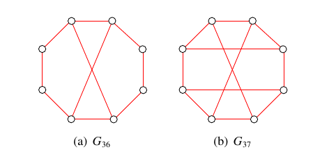
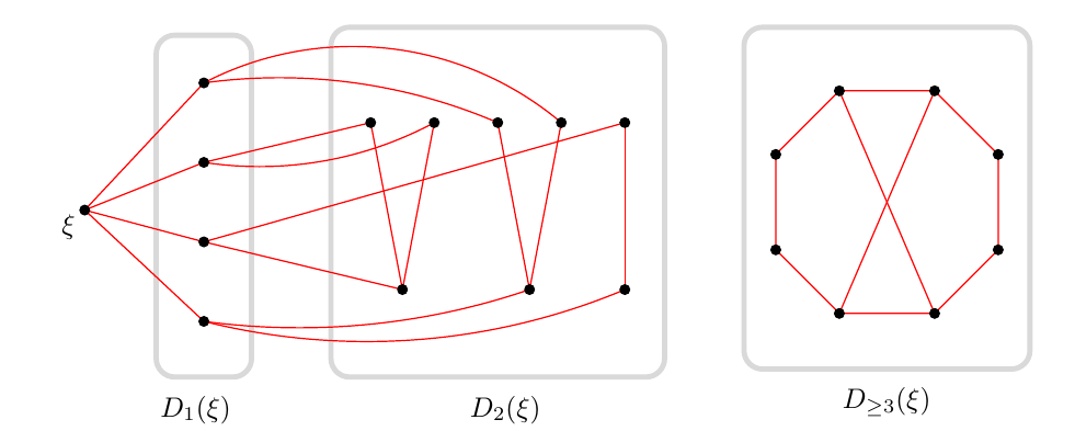
Consider, for example, Subcase IVb(viii) in Table 7. An example of a result obtained upon having applied the first three steps of our four-step enumeration process in this case (i.e. before the branching of Step 4 commences) is shown in Figure 10. Note that one of the two possible \(t(3,4,8)\) colourings in Figure 5, namely \(G_{36}\), appears as \(\langle D_{\geq 3}(\xi)\rangle_{{\rm red}}\) in Figure 10. All non-red edges entirely within the sets \(D_1(\xi)\), \(D_2(\xi)\) and \(D_3(\xi)\) are blue, and so are the edges between \(\xi\) and \(D_2(\xi)\), between \(\xi\) and \(D_3(\xi)\), and between \(D_1(\xi)\) and \(D_3(\xi)\). Branching occurs only on the remaining edges between \(D_1(\xi)\) and \(D_2(\xi)\) as well as on the edges between \(D_2(\xi)\) and \(D_3(\xi)\), eventually resulting in the \(t(3,8,21)\) colouring \(H_3\) shown in Figure 11.
Suppose now \(\Delta(\Xi)=5\). Then \(|D_2(\xi)|\leq 11\) and \(|D_{>2}(\xi)|<t(3,3)=6\) by Lemma 5. Furthermore, we have the following restriction on the number of small components in \(\langle D_{2}(\xi)\rangle_{{\rm red}}\).
Lemma 8. If \(|X|=6\), \(|Y|=4\), \(\Delta(\Xi)=5\) and \(\langle D_{>2}(\xi)\rangle_{{\rm red}}\) has exactly two \((1,0)\) components, then \(\langle D_{2}(\xi)\rangle_{{\rm red}}\) is not a subgraph of \(\Xi\).
Proof. By contradiction. Suppose, to the contrary, that \(|X|=6\), \(|Y|=4\), \(\Delta(\Xi)=5\) and \(\langle D_{>2}(\xi)\rangle_{{\rm red}}\) has exactly two \((1,0)\) components, but that \(\langle D_{2}(\xi)\rangle_{{\rm red}}\) is a subgraph of \(\Xi\). It follows from Observation 2 that \(D_{>3}(\xi)=\emptyset\) and hence from Observation 2 that \(\langle D_3(\xi)\rangle_{{\rm red}}\) is the red subgraph of a \(t(3,3,5)\) colouring. Furthermore, each vertex \(v\in D_3(\xi)\) is joined to a \((1,0)\) component by a red edge, for otherwise \(\langle \{\xi,v\}\cup D_{2}(\xi)\rangle_{{\rm blue}}\) contains a clique of order \(8\). Consequently one of the \((1,0)\) components is joined to at least three vertices of \(D_3(\xi)\) by red edges. These three vertices form a triangle in \(\langle D_{3}(\xi)\rangle_{{\rm blue}}\) in order to avoid forming a triangle in \(\Xi\), but this contradicts the fact that \(\langle D_3(\xi)\rangle_{{\rm red}}\) is the red subgraph of a \(t(3,3,5)\) colouring. ◻
The results obtained upon having applied our four-step enumeration process of §4.1 to subcases V–VIb in Table 4 are presented in [21, Tables 15-17].
It is known that there is only one \(t(3,3,5)\) colouring, two \(t(3,4,8)\) colourings, six \(t(3,5,11)\) colourings and thirty four \(t(3,6,14)\) colourings [6, Table 3]. We validated our computer implementation of the four-step enumeration process described in §4.1 by verifying these results independently. We also verified that the results obtained by this process are independent of the choice of the vertex \(\xi\) in each case.
A total of 298 \(t(3,7,17)\) colourings were uncovered during the enumeration process described in the previous sections. These colourings have not been enumerated before and are available online [22].
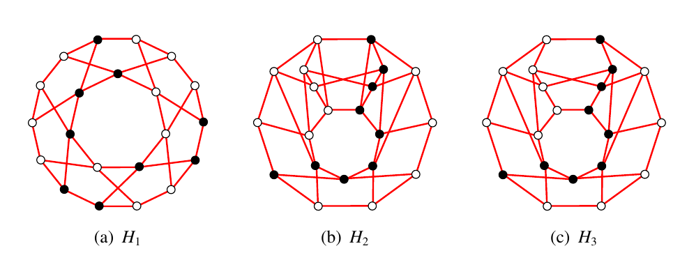
Furthermore, a total of six \(t(3,8,21)\) colourings were similarly found, as summarised in [21]. Among these colourings there are, however, only three pairwise non-isomorphic colourings — all corresponding to the case where \(\Delta(\Xi)=4\). The red subgraphs of these colourings are shown in Figure 11.
Since the circulant graph \(R\) in Figure 12(a) contains no irredundant set of cardinality \(8\) and the circulant graph \(B\) in Figure 12(b) contains no irredundant set of cardinality \(3\), it follows that the pair \((R,B)\) in Figure 12 forms an \(s(3,8,20)\) colouring.
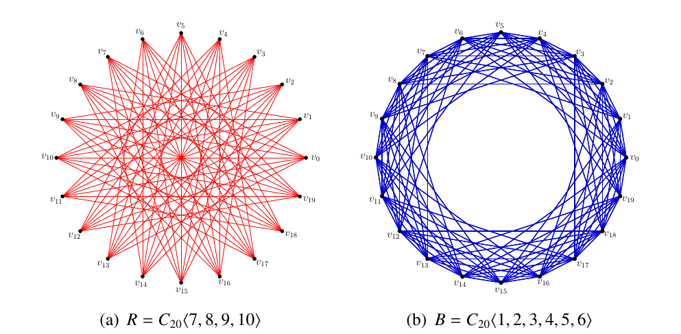
It therefore follows by (2) and Table 1 that \[21 \leq s(3,8) \leq w(3,8) \leq t(3,8)=22. \label{bestbounds}\tag{4}\] Lemma 2 implies that sets of \(s(3,8,21)\) and \(w(3,8,21)\) colourings may be found from among the set of \(t(3,8,21)\) colourings enumerated in §4. The graphs in Figure 11 each contains a minimal dominating (or maximal irredundant) set of cardinality \(9\), so that none of these graphs represent \(w(3,8,21)\) colourings, or \(s(3,8,21)\) colourings, and hence we have the following result in view of (4).
Theorem 3. \(s(3,8)=w(3,8)=21\).
In order to pave the way for the computation of the Ramsey numbers \(s(3,9)\) and \(t(3,9)\), we establish the following bounds.
Theorem 4. \(24\leq s(3,9)\leq t(3,9)\leq 27\).
Proof. Using the notation introduced in Figure 12, the circulant graph \(R'=C_{23}\langle8,9,10,11\rangle\) contains no irredundant set of cardinality \(9\) and the circulant graph \(B'=C_{23}\langle1,2,3,4,5,6,7\rangle\) contains no irredundant set of cardinality \(3\). The pair \((R',B')\) therefore forms an \(s(3,9,23)\) colouring and hence \(s(3,9)\geq 24\).
In order to establish the desired upper bound on \(t(3,9)\), we show by contradiction that no \(t(3,9,27)\) colouring exists. Suppose, to the contrary, that such a colouring indeed exists, and let \(\Xi'\) be its red subgraph. Then it follows from Corollary 2 that \(\delta(\Xi')\geq 27-t(3,8)=27-22=5\). It also follows from Corollary 1 that \(\Delta(\Xi')<t(2,9)=9\), and so \(\Delta(\Xi')=5\), \(6\), \(7\) or \(8\).
Let \(v\) be a vertex of maximum degree in \(\Xi'\) and suppose \(\Delta(\Xi')=8\). Then \(D_{\geq 3}(v)\) is empty in order to avoid a clique of order \(9\) in the blue subgraph \(\overline{\Xi'}\). But then \(D_2(v)\) has cardinality \(18\) and forms a clique of order \(9\) in \(\overline{\Xi'}\) by Lemma 4(b), a contradiction.
Suppose next that \(v\) has degree \(6\) or \(7\). Then by an argument similar to the one above, we may assume that \(D_3(v)\) is not empty (so as to avoid a large set \(D_2(v)\)). But then it follows from Lemma 4(b) that \(D_2(v)\) has fewer than \(14\) vertices in order to avoid a clique of order \(9\) in \(\overline{\Xi'}\) (on the vertices of a partite set of the bipartite graph in \(D_{\geq 2}(v)\) together with \(v\)). Furthermore, similar to Observation 2, we also have that \(D_{\geq3}(v)\) has fewer than \(t(3,9-\Delta(\Xi'))\) vertices, and so \(\Xi'\) has fewer than \(1+\Delta(\Xi')+13+t(3,9-\Delta(\Xi'))\) vertices. For \(\Delta(\Xi')=6\) or \(7\), this value is \(25\) or \(24\), respectively — contradicting the fact that \(\Xi'\) has order \(27\).
It follows that \(\Xi'\) is a \(5\)-regular graph, which is a contradiction, because it has odd order. ◻
As further work, we propose that the values of \(s(3,9)\) and \(t(3,9)\) be computed according to our enumeration strategy in §4.1. In order to render this strategy feasible for graphs of orders \(24\)–\(27\), however, we anticipate that our branch-and-bound procedure in §3 will have to be refined, possibly by selecting the branching order judiciously. We furthermore expect that the development of new theoretical results will be required in order to extend the bounding list of Table 6.
The authors declare that they have no known competing financial interests or personal relationships that could have appeared to influence the work reported in this paper.