A graceful labeling of a tree \(T\) of order \(n\) is a bijection \(f:V(T) \rightarrow \{0, 1, \dots, n-1\}\) that induces on each edge \(uv\) a weight given by \(|f(u)-f(v)|\) and the set of weights is \(\{1, 2, \dots, n-1\}.\) If such a labeling exists, the tree \(T\) is said to be graceful. The complementary labeling of \(f,\) denoted by \(\overline{f},\) is the function defined for every \(v \in V(T)\) as \(\overline{f}(v)=n-1-f(v).\) A labeling \(h\) of \(T\) is a shifting of \(f\) in \(c\) units if \(h(v)=f(v)+c\) for every \(v \in V(T).\) Note that \(f,\) \(\overline{f},\) and \(h\) have the same set of induced weights. Let \(A\) and \(B\) be the stable sets of \(T,\) a graceful labeling \(f\) of \(T\) is said to be an \(\alpha\text{-labeling}\) of \(T,\) if for every \((u, v) \in A \times B,\) \(f(u) < f(v),\) i.e., the smaller labels are assigned to the vertices in \(A;\) the boundary value of \(f\) is \(\lambda=\text{max}\{f(u):u \in A\}.\) If such a labeling exists, then \(T\) is called an \(\alpha\text{-tree}\). We refer to the elements of \(A\) and \(B\) as the dark and light vertices, respectively. If \(f\) is an \(\alpha\text{-labeling}\) of \(T,\) then \(\overline{f}\) is also an \(\alpha\text{-labeling}\) of \(T\) but its boundary value is \(n-1-\lambda.\) There is another \(\alpha\text{-labeling}\) of \(T\) associated with \(f,\) denoted by \(f_r,\) called its reverse labeling, this function is defined for every \(v \in V(T)\) as \(f_r(v)=\lambda-f(v)\) if \(v \in A\) and \(f_r(v)=n+\lambda-f(v)\) if \(v \in B.\) Note that \(f\) and \(f_r\) have the same boundary value. Graceful and \(\alpha\text{-labelings}\) were introduced by Rosa [6] with the names of \(\beta\text{-}\) and \(\alpha\text{-valuations}\), respectively. The concept of reverse labeling was also given by Rosa [7], he called it inverse labeling. A labeling \(f\) of \(T\) is said to be bipartite if the labels of the dark vertices are smaller than the labels of the light vertices. Thus, an \(\alpha\text{-labeling}\) is a bipartite graceful labeling.
Suppose that \(f\) is an \(\alpha\text{-labeling}\) of \(T\) and \(d\) is a positive integer; let \(g\) be the labeling of \(T\) defined for every \(v \in V(T)\) as \(g(v)=f(v)\) when \(v \in A\) and \(g(v)=d-1+f(v)\) when \(v \in B.\) This transformed \(\alpha\text{-labeling}\) is called \(d\text{-graceful labeling}\). The labeling \(g\) assigns to the elements of \(A\) the labels in \([0, \lambda]\) and to the elements of \(B\) the labels in \([d+\lambda, d+n-2];\) since \(f\) is an \(\alpha\text{-labeling}\), for each \(w \in \{1, 2, \dots, n-1\},\) there exists an edge \(uv\) in \(T,\) with \((u, v) \in A \times B\) such that \(f(v)-f(u)=w,\) then \(g(v)-g(u)=d-1+f(v)-f(u)=d-1+w,\) since \(1 \leq w \leq n-1,\) we conclude that the set of weights induced by \(g\) is \(\{d, d+1, \dots, d+n-2\}.\) This characteristic of the \(\alpha\text{-labeling},\) \(f,\) has been used extensively in the construction of new \(\alpha\text{-trees}\) and it is essential in this work.
In the last decades, several methods to construct graceful and \(\alpha\text{-trees}\) have been investigated. An important number of these methods is associated with the vertex amalgamation, where two trees are merged by identifying two of their vertices. A few years after Rosa introduced these labelings, Stanton and Zarnke [8] presented a method where a graceful tree is obtained, they started with two graceful trees \(S\) (called the host) and \(T,\) the new graceful tree was obtained, by attaching to every vertex of the host a copy of \(T.\) Years later, Koh et al. [4] extended the result of Stanton and Zarnke by proving that different \(\alpha\text{-trees}\) can be attached to the vertices of \(S;\) if the vertices of \(S\) are named \(1, 2, \dots, n,\) they amalgamated the vertices \(i\) and \(n+1-i\) with a pair of distinguished vertices of two \(\alpha\text{-trees}\), designated as \(T_1\) and \(T_2,\) such that their stable sets satisfy \(|A_1|=|A_2|\) and \(|B_1|=|B_2|.\) In [5], Mavronicolas and Michael, showed that the vertex labeled \(i\) in \(S\) can be amalgamated with the vertex labeled 0 in \(T_i,\) where each \(T_i\) is an \(\alpha\text{-labeled}\) tree with boundary value \(\lambda\) and order \(n;\) we must take into account, that in the work of these authors, \(T_i\) and \(T_j\) are not necessarily isomorphic.
In the present study, we do something similar to what all these authors did before, but with some important differences. First, the host is a path-like tree (a tree originated from a path by moving some edges) or a special type of caterpillar (a caterpillar where all the internal vertices have the same degree), we prove that any pair \(v_i\) and \(v_{i+1}\) of adjacent vertices, where \(v_i\) and \(v_{i+1}\) are on the longest path, can be amalgamated with the vertices labeled 0 of two \(\alpha\text{-labeled}\) trees of the same size and boundary value. These amalgamations can be done for any number of pairs of adjacent vertices, with the only restriction that each vertex on the longest path can be used at most once in these amalgamations. In this way, the main differences with the previous related results is that we can choose where to do the amalgamations and the trees attached to the host may have different sizes.
In [6], Rosa proved that all caterpillars are \(\alpha\text{-graphs}\). When the caterpillar is a path, the labeling \(f\) given by Rosa follows the pattern shown in Figure 1.
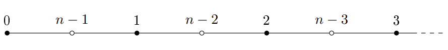
The regularity exhibited by both, the path and this labeling, motivates us to explore different ways to construct gracefully labeled graphs by preserving the characteristic of the labeling and modifying the structure of the graph. Through this entire work we use \(V(P_n)=\{v_1, v_2, \dots, v_n\}\) and \(E(P_n)=\{v_iv_{i+1}: 1 \leq i \leq n-1\}.\) Let \(a, b \in \{1, 2, \dots, n\},\) with \(a < b.\) Note that if \(a\) and \(b\) have the same parity, then \(f(v_a)=f(v_b)-\frac{b-a}{2}\) when \(a\) is odd and \(f(v_a)=f(v_b)+\frac{b-a}{2}\) when \(a\) is even. Let \(w\) be the weight of the edge \(v_iv_{i+1}\) under the labeling \(f,\) then one of the following equations must hold:
\[ f(v_i)-f(v_{i+1})=w,\label{eq1}\ \tag{1}\] \[f(v_{i+1})-f(v_i)=w.\ \tag{2}\]
Note that Eq. (1) holds, i.e., if \(i\) is even and Eq. (2) holds, i.e., if \(i\) is odd.
Suppose that there exists a positive integer \(x,\) such that \(i-x \geq1\) and \(i+1+x \leq n.\) If \(x\) is even and Eq. (1) holds, then \[\begin{aligned} f(v_{i-x})-f(v_{i+1+x})&=\Big(f(v_i)+\frac{i-(i-x)}{2}\Big)-\Big(f(v_{i+1})+\frac{i+1+x-(i+1)}{2}\Big)\\ &=f(v_i)+\frac{x}{2}-f(v_{i+1})-\frac{x}{2}\\ &=f(v_i)-f(v_{i+1})=w. \end{aligned}\]
If Eq. (2) holds, then \[\begin{aligned} f(v_{i+1+x})-f(v_{i-x})&=f(v_{i+1})-\frac{x}{2}-\Big(f(v_{i})-\frac{x}{2}\Big)\\ &=f(v_{i+1})-\frac{x}{2}-f(v_{i})+\frac{x}{2}\\ &=f(v_{i+1})-f(v_{i})=w. \end{aligned}\]
Suppose now that \(x\) is odd. If Eq. (1) holds, then \[\begin{aligned} f(v_{i-x})-f(v_{i+1+x})&=f(v_{i+1})-\frac{x+1}{2}-\Big(f(v_{i})-\frac{x+1}{2}\Big)\\ &=f(v_{i+1})-f(v_{i})=w. \end{aligned}\]
If Eq. (2) holds, then \[\begin{aligned} f(v_{i+1+x})-f(v_{i-x})&=f(v_{i})+\frac{x+1}{2}-\Big(f(v_{i+1})+\frac{x+1}{2}\Big)\\ &=f(v_{i})-f(v_{i+1})=w. \end{aligned}\]
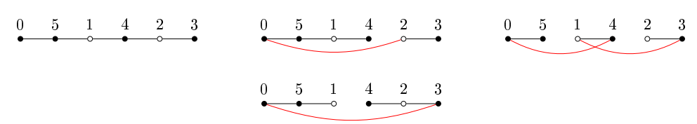
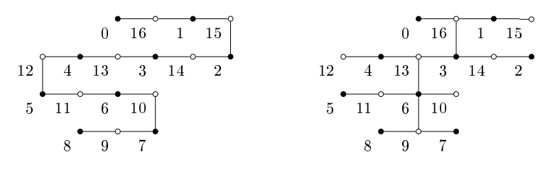
Thus, regardless the parity of \(x,\) we have that \(f(v_{i-x})-f(v_{i+1+x})=w.\) Therefore, the edge \(v_iv_{i+1}\) of \(P_n\) can be replaced by a new edge of weight \(w,\) obtained by connecting the vertices \(v_{i-x}\) and \(v_{i+1+x}.\) Since the labels have not been modified in any way, this new tree is \(\alpha\text{-labeled.}\) Any tree obtained after a sequence of these replacements is called a path-like tree. It was proven in [1] that all path-like trees are \(\alpha\text{-trees.}\) Note that when \(n\) is even and \(x=\frac{n}{2},\) the graph obtained with the replacement of the central edge of \(P_n,\) is \(P_n\) itself, but with a different \(\alpha\text{-labeling.}\) Of course this is not the only way to obtain other \(\alpha\text{-labelings}\) of \(P_n,\) consider the examples, of \(\alpha\text{-labelings}\) of \(P_6\) obtained with this method, shown in Figure 2.
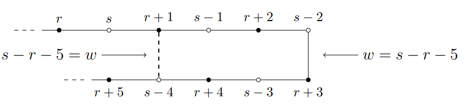
There is a more intuitive way to see a path-like tree. Let \(n_1\) and \(n_2\) be positive integers larger than 2 such that \(n_1+n_2=n.\) Suppose that \(v_1, v_2, \dots, v_{n_1}\) are placed on the points of the integral grid with coordinates \((1,1), (2,1), \dots, (n_1, 1),\) respectively, and \(v_{n_1+1}, v_{n_1+2}, \dots, v_{n_1+n_2}\) are on the points with coordinates \((n_1, 0), (n_1-1, 0), \dots, (n_1-n_2+1, 0),\) respectively. The edge \(v_{n_1}v_{n_1+1}\) of \(P_n\) is the only one connecting a vertex on the line \(y=1\) with a vertex on the line \(y=0.\) This edge can be moved to the left \(x\) units and the new edge has the same weight than \(v_{n_1}v_{n_1+1}.\) We show this fact in Figure 3, where \(r \ll s.\)
Certainly, we can choose \(n_1+n_2+ \cdots + n_k=n,\) where \(n_i \geq 2,\) and position the vertices of each subpath \(P_{n_i}\) on the line \(y=k-i\) in such a way that when all the vertices are in place, the path \(P_n\) forms a \(90^{\circ}\) angle zig-zag. Thus, each path-like tree \(T\) is associated with a \(k\text{-part}\) partition of \(n,\) that induces the subpaths \(P_{n_i}.\) Suppose that \(T\) is any path-like tree obtained from \(P_n;\) let \(v_1, v_2, \dots, v_n\) be the consecutive vertices of \(P_n,\) we say that \(v_j\) is a bending point of both \(P_n\) and \(T\) if \(j\) is either \(\tilde{n}_i\) or \(\tilde{n}_i+1,\) where \(\tilde{n}_i=\sum_{j=1}^in_j.\) Note that the number of bending points on \(T\) is always even, in particular, if \(n_1+n_2+ \cdots + n_k=n,\) \(T\) has exactly \(2(k-1)\) of these points; the bending points \(v_i\) and \(v_{i+1}\) form a tandem if \(v_i\) lies on \(y=k-i\) and \(v_{i+1}\) lies on \(y=k-i-1.\) These vertices, together with \(v_1\) and \(v_n,\) play an important role in our main theorem. In Figure 4 we show an example of an embedding on the integral grid of the path \(P_{17},\) where \(n_1=4, n_2=6, n_3=4\) and \(n_4=3,\) together with a path-like tree, \(T,\) obtained from the embedding. The bending points are the vertices labeled 15, 2, 12, 5, 10, and 7. The number of non-isomorphic path-like trees that can be obtained from a given embedding of the path on the integral grid is substantial, for the embedding shown in this figure, there are 48 non-isomorphic path-like trees, including the path itself.
Suppose that for every \(i \in \{1, 2, \dots, k\},\) \(T_i\) is a tree of positive size. Let \(u_i\) and \(v_i\) be two distinct vertices of \(T_i.\) Consider the tree \(T\) obtained by amalgamating, for each \(2 \leq i \leq k-1,\) the vertex \(u_i\) to the vertex \(v_{i-1}\) and \(v_i\) to \(u_{i+1}.\) This tree \(T\) was called a chain tree in [2], in that work we proved that when all the \(T_i\)’s are \(\alpha\text{-trees,}\) there is a chain tree \(T\) built with these \(T_i\)’s that is also an \(\alpha\text{-tree.}\) For the sake of completeness, we prove here the special case where \(k=3.\) This restricted version of the result in [2] is used later in this paper, within the proof of Theorem 2.5. Recall that in an \(\alpha\text{-labeling}\) of a graph, the smaller labels are always assigned to the dark vertices; in addition, for an \(\alpha\text{-labeled}\) tree \(T_i,\) the positive integer \(\lambda_i\) is the boundary value of the associated \(\alpha\text{-labeling,}\) and \(n_i\) is the order of \(T_i.\)
Lemma 2.1. If \(T_1,\) \(T_2,\) and \(T_3\) are \(\alpha\text{-labeled}\) trees of positive size, then an \(\alpha\text{-tree}\) is obtained by amalgamating the vertex labeled \(\lambda_1\) in \(T_1\) to the vertex labeled 0 in \(T_2\) and the vertex labeled \(\lambda_2\) (resp. \(\lambda_2+1\)) in \(T_2\) to the vertex labeled 0 (resp. \(n_3\)) in \(T_3.\)
Proof. Suppose that for each \(i \in \{1, 2, 3\},\) \(T_i\) is an \(\alpha\text{-tree}\) of order \(n_i \geq 2.\) Let \(f_i\) be an \(\alpha\text{-labeling}\) of \(T_i.\) Thus, the dark vertices of \(T_i\) have their labels in the interval \([0, \lambda_i]\) and the light vertices in \([\lambda_i+1, n_i-1].\) Note that any chain tree obtained with these trees has order \(n_1+n_2+n_3-2.\)
Following the procedure mentioned in the Introduction, the labeling of \(T_1\) is transformed into a (\(n_2+n_3-1\))-graceful labeling; thus, the labels on the dark vertices are in \([0, \lambda_1],\) the labels on the light vertices are in \([\lambda_1+n_2+n_3-1, n_1+n_2+n_3-3],\) and the induced weights form the interval \([n_2+n_3-1, n_1+n_2+n_3-3].\)
Similarly, the labeling of \(T_2\) is transformed into a \(n_3\)-graceful labeling shifted \(\lambda_1\) units. Now, the labels on the dark vertices are in \([\lambda_1, \lambda_1+\lambda_2],\) the labels on the light vertices are in \([\lambda_1+\lambda_2+n_3, \lambda_1+n_2+n_3-2],\) and the induced weights are in \([n_3, n_2+n_3-2].\) Note that the label \(\lambda_1\) has been used on both \(T_1\) and \(T_2,\) consequently, we amalgamate the two vertices labeled \(\lambda.\)
Since there are two options to amalgamate \(T_2\) and \(T_3\) we analyze two cases. Suppose first that the labeling of \(T_3\) is shifted \(\lambda_1+\lambda_2\) units, the new labels of \(T_3\) are in \([\lambda_1+\lambda_2, \lambda_1+\lambda_2+n_3-1]\) and the induced weights are in \([1, n_3-1].\) In this case, \(T_2\) and \(T_3\) have a vertex labeled \(\lambda_1+\lambda_2,\) amalgamating the vertices with this label we create a labeled chain tree, where the labels are \(0, 1, \dots, n_1+n_2+n_3-3\) and the induced weights are \(1, 2, \dots, n_1+n_2+n_3-3.\) Since we always amalgamated vertices with the same color, the labeling is in fact an \(\alpha\text{-labeling.}\)
If the labeling of \(T_3\) is shifted \(\lambda_1+\lambda_2 +1\) units, then the new labels are in \([\lambda_1+\lambda_2 +1, \lambda_1+\lambda_2+n_3].\) Now \(T_2\) and \(T_3\) have a vertex labeled \(\lambda_1+\lambda_2 +n_3.\) We proceed as before amalgamating these two vertices to produce a chain tree with an \(\alpha\text{-labeling.}\) ◻
In Figure 5 we show an example of this construction, where each tree is drawn using different line colors.
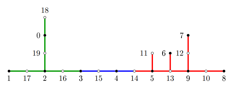
Remark 2.2. As we said before, an important characteristic of an \(\alpha\text{-labeling}\) is that it can be transformed into a \(d\text{-graceful}\) labeling. This fact was used on the labelings of \(T_1\) and \(T_2\) but not on the labeling of \(T_3,\) this implies that \(T_3\) may be replaced by any gracefully labeled tree. If this is the case, the final labeling of \(T\) is graceful.
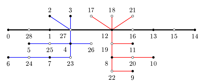
For \(i=1,2,\) let \(T_i\) be an \(\alpha\text{-tree}\) of order \(p\) whose stable sets are \(A_i\) and \(B_i.\) We say that \(T_1\) and \(T_2\) are equivalent if \(|A_1| = |A_2|.\) In other terms, two trees are said to be equivalent if their corresponding stable sets have the same cardinalities. Two equivalent trees of order 11 are shown in red and blue in Figure 6. The fact that \(T_i\) is an \(\alpha\text{-labeling}\) implies the existence of an \(\alpha\text{-labeling}\) of \(T_i\) that assigns the label 0 to a vertex of \(A_i.\)
Lemma 2.3. Let \(T_1\) and \(T_2\) be equivalent trees of order \(p.\) Suppose that \(f_i\) be an \(\alpha\text{-labeling}\) of \(T_i\) with boundary value \(\lambda_i.\) If \(\lambda_1=\lambda_2,\) then an \(\alpha\text{-tree}\) \(T\) is obtained by connecting with an edge the vertices labeled 0.
Proof. Suppose that \(T_i\) has been labeled using the function \(f_i.\) Let \(v_i\) denote the vertex of \(T_i\) labeled 0 by \(f_i.\) Since \(\lambda_1 = \lambda_2\), the vertices \(v_1\) and \(v_2\) are in stable sets with the same cardinality. For the sake of simplicity, let \(\lambda = \lambda_1.\) The tree \(T\) obtained by adding to \(T_1 \cup T_2\) the edge \(v_1v_2\) has size \(2p-1\) and its stable sets have cardinality \(p.\) In order to obtain an \(\alpha\text{-labeling}\) of \(T\) we proceed as follows:
Transform \(f_1\) into a \((p+1)\text{-graceful}\) labeling; in this way, the dark vertices have their labels in \([0, \lambda],\) the light vertices have their labels in \([\lambda+p+1, 2p-1],\) and the induced weights are in \([p, 2p-2].\)
In the case of \(T_2\), instead of using \(f_2\) we use the reverse of its complementary labeling shifted \(\lambda+1\) units. Let \(g\) be the reverse of \(\overline{f}_2\) shifted \(\lambda+1\) units, then \(g\) is defined for every \(v \in V(T_2)\) as \[g(v)= \begin{cases} p+f_2(v) &\text{ if }f_2(v)\leq \lambda,\\ f_2(v) &\text{ if }f_2(v) > \lambda. \end{cases}\]
Therefore, the weights induced by \(g\) are in \([1, p-1]\) and the labels in \([\lambda+1, p+\lambda].\) Consequently, there is no repetition of labels between \(T_1\) and \(T_2.\) Since \(f_2(v_2)=0,\) we know that \(g(v_2)=p+f_2(v_2)=p.\) Hence, if we connect \(v_1\) and \(v_2\) we create an edge of weight \(p.\) Thus, the weights on the edges of \(T\) are \(1, 2, \dots, 2p-1.\) Since the labelings used on \(T_1\) and \(T_2\) are bipartite, and the new edge connects vertices of different colors, the final labeling of \(T\) is indeed an \(\alpha\text{-labeling}.\) ◻
Recall that the tree \(T\) in Lemma 2.3 has order \(2p\) and each stable set has cardinality \(p;\) consequently, the \(\alpha\text{-labeling}\) \(f\) of this tree has boundary value \(\lambda=p-1.\) Since \(f(v_1)=0\) and \(f(v_2)=p,\) this labeled tree can be the tree \(T_2\) in Lemma 2.1, if we take \(T_1\) and \(T_3\) to be two paths, not necessarily isomorphic, each of them labeled with the labeling in Figure 1 or the associated complementary labeling, chosen to satisfy the conditions of Lemma 2.1, then we obtain a tree \(T\) where two equivalent trees have been attached to any two adjacent vertices of a path. In other terms, we have proven the following theorem.
Theorem 2.4. If the vertices labeled 0 of two equivalent \(\alpha\text{-labeled}\) trees are amalgamated with two adjacent vertices of a path, then the result of this amalgamation is an \(\alpha\text{-tree.}\)
In Figure 6 we show an example of a tree constructed by amalgamating equivalent \(\alpha\text{-trees}\) to two interior adjacent vertices of a path of order 9, which is represented with black edges while the trees \(T_1\) and \(T_3\) from Lemma 2.1 are represented with blue and red edges, respectively.
Since the labelings on \(T_1\) and \(T_3\) are, essentially, \(\alpha\text{-labelings,}\) it is possible to draw the \(\alpha\text{-tree}\) \(T\) from Lemma 2.3, as in Figure 3, in such a way that \(v_1\) and \(v_2,\) (i.e. the vertices where the equivalent trees were amalgamated), correspond to bending points. Therefore, the edge \(v_1v_2,\) that is the “vertical” edge in this representation, can be moved horizontally to create a new \(\alpha\text{-graph,}\) where the subgraph induced by the vertices of \(T_1\) and \(T_3\) is a path-like tree. Furthermore, the leaf of \(T\) that corresponds to the last vertex of the path \(T_3\) is labeled with the boundary value of the labeling of \(T\) or this value plus one. This implies that if \(T\) and \(T'\) are two trees obtained following the procedure in Lemma 2.3, we can amalgamate them through the first vertex of the first path in \(T'\) with the last vertex of the second path in \(T.\) This process can be repeated as many times as needed to form a path-like tree where any number of bending point tandems are amalgamated with the vertices labeled 0 of two \(\alpha\text{-labeled}\) equivalent trees. Hence, as a consequence of all the previous results we get the following theorem.
Theorem 2.5. Let \(T\) be a path-like tree of order \(n,\) \(S\) be the set of all tandems of bending points in \(T,\) and \(R \subseteq S.\) An \(\alpha\text{-tree}\) is obtained if for each \((v_i, v_{i+1}) \in R,\) the vertices \(v_i\) and \(v_{i+1}\) are amalgamated with the vertices labeled 0 in two \(\alpha\text{-labeled}\) equivalent trees.
Given the fact that the vertices \(v_1\) and \(v_n\) of \(T\) are not bending points and that \(v_1\) is labeled 0 or \(n\) while \(v_n\) is labeled with the boundary value or this value plus one, we can use \(T\) in the place of \(T_2\) in Lemma 2.1 and attach an \(\alpha\text{-tree}\) to each of these vertices to produce another \(\alpha\text{-labeled}\) tree. As we mentioned in Remark 2.2, we may use a graceful tree instead of an \(\alpha\text{-tree}\) in the place of \(T_3;\) in that case, the outcome is a new graceful tree. We show this fact in Figure 7, presenting a graceful tree built on the path-like tree in Figure 4.
Furthermore, the amalgamation of equivalent trees described in Theorem 2.4 can be done on any subpath of an \(\alpha\text{-tree}\) \(T\) provided that the \(\alpha\text{-labeling}\) of \(T\) restricted to this subpath follows the pattern described in Figure 3. In [3] we introduced several \(\alpha\text{-trees}\) obtained by attaching paths, which lengths form an arithmetic progression of difference 1, to the vertices of another path (the host), we refer to the resulting tree as a triangular tree. The labelings of each attached path follows the pattern in Figure 3, therefore triangular trees can be used, in the same way that path-like trees were used in Theorem 2.5, to form a broader class of trees that admit \(\alpha\text{-labelings.}\)
Before closing this work, we must observe that in general, in an \(\alpha\text{-tree,}\) there are at least four vertices that can be labeled 0. Indeed, if \(f\) is an \(\alpha\text{-labeling}\) with boundary value \(\lambda\) of a tree \(T\) of order \(n,\) there exist \(v_1, v_2, v_3, v_4 \in V(T)\) such that \(f(v_1)=0,\) \(f(v_2)=\lambda,\) \(f(v_3)=\lambda+1,\) and \(f(v_4)=n-1.\) Therefore, \(f_r(v_2)=0,\) \(\overline{f}_r(v_3)=0,\) and \(\overline{f}(v_4)=0.\) This property gives more strength to the results presented in this work. Another interesting property that makes these results even broader, is associated with the fact that a path can be seen as a caterpillar where the vertices on its spine have degree 2, then instead of using a path we can use a caterpillar where every vertex on its spine has degree \(r \geq 2.\) Suppose that \(v_i\) and \(v_{i+1}\) are two adjacent vertices on the spine of one of these caterpillars, Rosa’s \(\alpha\text{-labeling}\) of caterpillars allows us to replace the edge \(v_iv_{i+1}\) for the edge \(v_{i-x}v_{i+1+x}\) as we did to create a path-like tree.
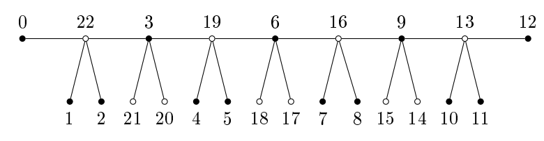
In Figure 8 we show Rosa’s \(\alpha\text{-labeling}\) of a caterpillar of order 23, where every internal vertex has degree 4. The weight on the “horizontal” edges form an arithmetic progression of difference 3, while on the \(\alpha\text{-labeling}\) of the path shown in Figure 1, the difference is 1.
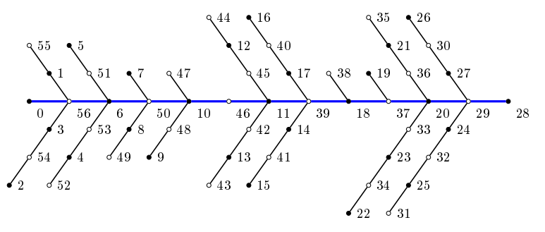
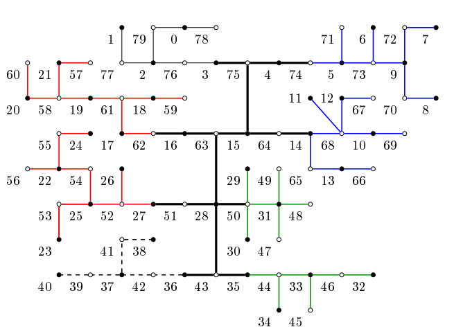
A weak aspect of this type of construction is that, sometimes, is not easy to determine whether a given tree can be built, following the steps of the construction. Among the trees that can be constructed, with the technique presented in Theorem 2.4, we have a class of trees of maximum degree 4. We say that a tree \(T,\) with maximum degree 4, is a fishbone tree if there is a path in \(T\) containing all vertices of degree larger than 2. In other terms, a fishbone tree is obtained by amalgamating vertices of a path (the spine) with vertices of other paths. In Figure 9 we show an \(\alpha\text{-labeling}\) of a fishbone tree of size 56, where the spine is the horizontal path. In [7], Rosa proved that there exists an \(\alpha\text{-labeling}\) of \(P_n\) that assigns the label 0 on any vertex \(v,\) except when \(v\) is the central vertex of \(P_5.\) Thus, if \(2k\) vertices of \(P_n\) are selected, say \(v_1, v_2, \dots, v_{2k},\) such that for each odd \(i \in \{1, 2, \dots, 2k\},\) \(v_iv_{i+1} \in E(P_n),\) then any fishbone tree obtained amalgamating \(v_i\) with any vertex \(u\) of a path \(P_{r_i}\) and \(v_{i+1}\) with the vertex \(u\) of a second copy of \(P_{r_i},\) except when \(P_{r_i} \cong P_5\) and \(u\) is its central vertex.