
The domination concept is commonly used to solve security and facility location concerns. The introduction of Roman domination resulted from studies into potential strategies for saving the Roman empire. The Italian domination was initiated as the improvement of Roman domination. In this paper, we introduce the inverse Italian dominating function in graphs.
The graphs used here are simple and cannot have isolated vertices. Two non-adjacent vertices \(v_1\) and \(v_2\) are said to be ‘identified’ if vertex \(v_1\) is deleted and all vertices adjacent to \(v_1\) are made adjacent to \(v_2\) [8]. An edge \(yz\) is said to be subdivided, if we remove the edge \(yz\) and add a new vertex \(x\) along with edges \(yx\) and \(xz\).
A vertex \(x\) in a tree is considered a descendant of a vertex \(y\) if \(y\) lies in the unique path that connects \(x\) to the root of the tree. The induced subgraph \(\left< S \right>\) where \(S\) contains a vertex \(u\) and its descendants is denoted by \(T_u\).
A set \(S \subseteq V\) in a graph \(G\) is called a dominating set if every vertex of \(G\) is either in \(S\) or adjacent to a vertex of \(S\). The domination number \(\gamma(G)\) equals the minimum cardinality of a dominating set in \(G\) [3]. Cockayne and Hedeteimi introduced this notation \(\gamma(G)\) in [3] for the domination number which is widely accepted now. The books [10] and [9] can be referred for more details.
Kulli and Sigarkanti introduced the concept of inverse dominating set in [12]. ‘‘Let \(S\) be a minimum dominating set of \(G\). If \(V – S\) contains a dominating set \(S{'}\) of \(G\), then \(S{'}\) is called an inverse dominating set of \(G\) with respect to \(S\). The inverse domination number of \(G\) is the minimum cardinality of an inverse dominating set of \(G\), denoted by \(\gamma_i(G)\) [12].’’
A dominating set \(D\) of a graph \(G\), is said to be a two dominating set of \(G\), if every vertex in \(V-D\) is adjacent to at least two vertices of \(D\). A minimum two dominating set is denoted by \(\gamma_2\) – set.
In \(2016\), Chellali et al. published [2] in which he introduced the Roman \(\{2\}\)-dominating function, which is now known as the Italian dominating function (IDF). ‘‘An IDF is a function \(f : V(G) \rightarrow \{0, 1, 2\}\) where every vertex \(v\) labeled \(0\) must satisfy \(\sum_{u \in N(v)}f(u) \geq 2\). The weight of \(f\) denoted by \(w(f)\) is equal to the sum of all of its labelings. The Italian domination number (IDN) of \(G\) is the minimum weight among them. It is denoted by \(\gamma_I(G)\) [2].’’An IDF with weight \(\gamma_I(G)\) is called a \(\gamma_{I}\) -function . Let \(V_0,V_1,V_2\) be the set of vertices with label \(0,1\) and \(2\) respectively under an IDF.
If \(f\) is a \(\gamma_I\) – function of \(G\), then \(S=\left \{ v \in V: f(v) > 0 \right \}\) is the corresponding \(\gamma_I\) – set of \(f\). We define another Italian dominating function \(f': V(G) \rightarrow \{0, 1, 2\}\), such that \(f'(v) = 0\) for all \(v \in S\). This is an inverse Italian dominating function (IIDF) of \(f\). We find IDFs \(f_i\) and its corresponding IIDF \(f_{ij}\) of the graph. The inverse Italian domination number \(\gamma_{iI}(G)\) of the graph \(G\) is given by \(\gamma_{iI}(G)=min\{w(f_{ij}) : i>0, j>0\}\). An IIDF that has a weight of \(\gamma_{iI}(G)\) is referred to as a \(\gamma_{iI}\) -function.
Some graphs, like \(K_1\), do not have IIDF for any \(\gamma_{I}\) -function. The graph \(K_2\) does not have an IIDF for the \(\gamma_{I}\) -function which assigns \(1\) to every vertex, where as it has an IIDF of weight \(2\) if the \(\gamma_{I}\) -function assigns \(2\) to one vertex and \(0\) to another. Figure 1 shows few IDF and IIDF of \(K_{4,5}\). In this Figure 1, \(f_1\) is an IDF and \(f_{11}, f_{12}, f_{13}, f_{14}, f_{15}, f_{16}, f_{17}\) are few minimum IIDF of \(f_1\). Furthermore, \(f_2\) is an IDF and \(f_{21}\) is the only possible IIDF of \(f_2\). We observe that, \(w(f_{11})=w(f_{12})=w(f_{13})=w(f_{14})=w(f_{15})=w(f_{16})=w(f_{17})=4\) and \(w(f_{21})=5\). We find all \(\gamma_{I}\) -functions \(f_i\) and its corresponding IIDFs \(f_{ij}\). The lowest weight among all IIDF is \(\gamma_{iI}(G)\). In this example \(\gamma_{iI}(K_{4,5})=4\).

Proposition 2.1 . i) For any \(K_n\) with \(n\geq 2\), \(\gamma_{I}(K_n) = \gamma_{iI}(K_n)=2\);
ii) For any \(P_{n}\), \(n>3\), \(\gamma_{iI}(P_n)=\left \lceil \frac{ n+2}{2} \right \rceil\);
iii) For any \(C_{n}\), \(n>3\),\(\gamma_{iI}(C_n)=\left\{\begin{matrix} \frac{n}{2}& \text{if $n$ is even}\\ \frac{n+3}{2}& \text{if $n$ is odd} \end{matrix}\right.\);
iv) For any \(K_{r, s}\) where \(s \geq r > 3\), \(\gamma_{I}(K_{r, s}) =\gamma_{iI}(K_{r, s})=4\);
v) For any \(K_{1,n-1}\) with \(n > 2\), \(\gamma_{iI}(K_{1,n-1}) = n- 1\).
Proposition 2.2. A graph \(G\) does not have an IIDF if \(G\) has an isolated vertex or there exists no \(\gamma_I\) -set of \(G\) which is a proper subset of \(V(G).\)
Proof. Let \(G\) be a graph that has an isolated vertex \(v.\) Then \(f(v)>0\) for any \(\gamma_I\) -function \(f\). If there exists any IIDF \(f^{'}\), then \(f^{'}(v)=0\) and as \(v\) is isolated, it is not dominated by any other vertex. Hence, we can not define an IIDF.
Let \(G\) be a graph having no \(\gamma_I\) -set of \(G\) which is a proper subset of \(V(G)\). If there exists any IIDF \(f^{'}\), then \(f^{'}(x)=0\) for all \(x\in V(G)\). Hence, we can not define an IIDF. ◻
Proposition 2.3. If \(G = K_{1}+M\), then \(\gamma_{iI}(G) = \gamma_{I}(M)\) for any graph \(M\).
Proof. Let \(f\) be a \(\gamma_{I}\) -function such that \(K_1\) is assigned \(2\) and \(0\) is assigned to the remaining vertices. In any minimum IIDF \(f^{'}\), \(K_1\) is assigned \(0\) which gives \(\gamma_{iI}(G) = \gamma_{I}(M)\). ◻
The characterization of \(\gamma_{I}(G)=2\) is given by Volkmann [15] as a corollary of a theorem. In this section we have given a proof for the same. We also characterize the graphs with \(\gamma_{I}(G)=3\). Using these results, we characterize the graphs having \(\gamma_{iI}(G)=2,3.\)
Theorem 3.1. [15] For any connected graph \(G\) and for graph \(H\), \(\gamma_I(G)=2\) if and only if \(G\cong K_1+H\) or \(G\cong \overline{K_2} +H\).
Proof. If \(\gamma_I(G)=2\), then either \(\left |V_2 \right |=1\) or \(\left |V_2 \right |=0\) and \(\left |V_1 \right |=2\). If \(\left |V_2 \right |=1\), then all vertices should be adjacent to the vertex labelled \(2\). Hence \(G\cong K_1+H\). If \(\left |V_2 \right |=0\) and \(\left |V_1 \right |=2\), then all vertices should be adjacent to two vertices \(x\) and \(y\) of \(V_1\). If the vertices \(x\) and \(y\) are adjacent, then \(G\cong K_1+H\). If \(x\) and \(y\) are not adjacent, then \(G\cong \overline{K_2} +H\).
Conversely, if \(G\cong K_1+H\), then the only minimum \(\gamma_{I}(G)\) assigns \(2\) to vertex \(K_1\) and the remaining vertices can be assigned \(0\) which gives \(\gamma_I(G)=2\). If \(G\cong \overline{K_2} +H\), then vertices of \(\overline{K_2}\) are assigned \(1\) and the vertices of \(H\) can be assigned \(0\).
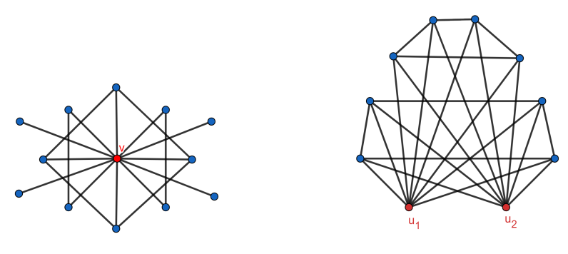
The Figure 2 shows graphs having \(\gamma_{I}(G)=2\). The vertex \(v\) of the first graph is of degree \(n-1\). The second graph is \(\overline{K_2} +H\) where \(u_1\), \(u_2\) forms \(\overline{K_2}\). ◻
Theorem 3.2. For any connected graph \(G\), \(\gamma_I(G)=3\) if and only if it satisfies any of the following properties:
i) \(\Delta(G)=n-2\) where \(G \ncong \overline{K_2}+H\) for any graph \(H\)
ii) \(G\) has a \(\gamma_2\) – set \(S\) with \(\left |S \right |=3\) where \(\Delta(G)< n-2\).
Proof. If \(\gamma_I(G)=3\), then either \(\left |V_2 \right |=1\) and \(\left |V_1 \right |=1\) or \(\left |V_2 \right |=0\) and \(\left |V_1 \right |=3\). If \(\left |V_2 \right |=1\) and \(\left |V_1 \right |=1\), then all vertices
are adjacent to the vertex labelled \(2\) except one, which implies \(\Delta(G)=n-2\). Furthermore, \(G \neq \overline{K_2}+H\) otherwise \(\gamma_I(G)=2\). If \(\left |V_2 \right |=0\) and \(\left |V_1 \right |=3\), then all the
vertices not in \(V_1\) should be
adjacent to any two vertices of \(V_1\)
which makes \(V_1\) a two dominating
set of \(G\). This two dominating set
is \(\gamma_2\) – set because if there
is a \(\gamma_2\) – set of cardinality
\(2\), then \(\gamma_I(G)=2\).
Conversely, if \(\Delta(G)=n-2\) with
\(G \neq \overline{K_2}+H\), then the
vertex with degree \(n-2\) can be
assigned \(2\) and the vertex not
adjacent to it can be assigned \(1\),
which gives \(\gamma_I(G)=3\). If there
is a \(\gamma_2\) – set \(S\) of \(G\) with \(\left
|S \right |=3\), then the vertices of \(S\) can be assigned \(1\) which gives \(\gamma_I(G)=3\).
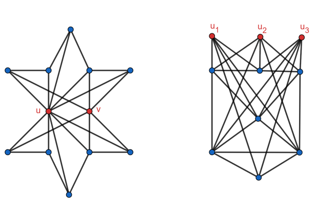
The Figure 3 shows the graphs having \(\gamma_{I}(G)\) equal to 3. In the first graph, \(u\) is the vertex of degree \(n-2\) and \(v\) is the vertex not adjacent to \(u\). In the second graph \(\{u_1,u_2,u_3\}\) form the \(\gamma_2\) – set of the graph. ◻
Theorem 3.3. For any connected graph \(G\), \(\gamma_{iI}(G)=2\) if and only if it satisfies any of the following properties:
i) \(G\cong K_2+H,\)
ii) \(G\cong P_3+H,\)
iii) \(G\cong
C_4+H,\)
for any graph \(H\).
Proof. For any connected graph \(G\), \(\gamma_{iI}(G)=2\) if and only if \(\gamma_{I}(G)=2\). From Theorem 3.1, we have, \(\gamma_I(G)=2\) if and only if \(G\cong K_1+M\) or \(G\cong \overline{K_2} +M\) for any graph \(M\).
Case 1. When \(G\cong K_1+M\).
If \(G\cong K_1+M\), then by Proposition 2.3, \(\gamma_{iI}(G)=\gamma_{I}(M)\) and \(\gamma_{I}(M)=2\) if and only if \(M=K_1+M_1\) or \(M \cong \overline{K_2} +M_2\) for any graphs \(M_1\) and \(M_2\). If \(G\cong K_1+M\) and \(M\cong K_1+M_1\), then \(G\cong K_2+H\) for some graph \(H\). If \(G\cong K_1+M\) and \(M\cong \overline{K_2} +M_2\), then \(G\cong P_3+H\) for some graph \(H\).
Case 2. When \(G\cong \overline{K_2} +M\).
In this case, \(\gamma_{iI}(G)=\gamma_I(M)\) and \(\gamma_{I}(M)=2\) if and only if \(M\cong K_1+H_1\) or \(M\cong \overline{K_2} +H_2\) for any graphs \(H_1\) and \(H_2\). If \(G\cong \overline{K_2} +M\) and \(M\cong K_1+H_1\), then \(G\cong P_3+H\) for some graph \(H\). If \(G\cong \overline{K_2} +M\) and \(M\cong \overline{K_2} +H_2\), then \(G\cong C_4+H\) for some graph \(H\).
Conversely, Suppose \(G\cong K_2+H\), then one vertex of \(K_2\) will be labelled \(2\) under any \(\gamma_{I}\) – function and the rest will be labelled \(0\). The IIDF will assign \(2\) to another vertex of \(K_2\) and the rest will be labelled \(0\). If \(G\cong P_3+H\), then the vertex with degree \(n-1\) is labelled \(2\) under any \(\gamma_{I}\) – function and the rest will be labelled \(0\). The IIDF will assign \(1\) to the vertices of \(P_3\) having degree \(n-2\) and the rest will be labelled \(0\). If \(G\cong C_4+H\), then any \(\gamma_{I}\) – function will assign \(1\) to two non-adjacent vertices of \(C_4\) and the rest will be labelled \(0\). Any IIDF will assign \(1\) to the other two non-adjacent vertices of \(C_4\) and the rest will be labelled \(0\). In all the above cases we get \(\gamma_{iI}(G)=2\).
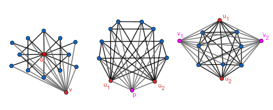
The Figure 4 shows the graphs (i) \(G\cong K_2+H\), (ii) \(G\cong P_3+H,\) and (iii) \(G\cong C_4+H,\) respectively. In the first graph \(u\) and \(v\) forms \(K_2\). In the second graph \(u_1,p,u_2\) forms \(P_3\). In the third graph \(v_1,v_2,u_1,u_2\) forms \(C_4\). ◻
Theorem 3.4. For any connected graph \(G\) with \(n \geq 3\), \(\gamma_{iI}(G)=3\) if and only if it satisfies any of the following properties:
i) \(G\cong K_1+H\) or \(G\cong \overline{K_2}+H\), where \(\Delta(H)=\left| V(H) \right|-2\) and \(H \ncong \overline{K_2} +M\) for any graph \(M\) and \(H\),
ii) \(G\cong K_1+H\) or \(G\cong \overline{K_2}+H\), where \(H\) has a \(\gamma_2\) – set \(S\) with \(\left| S \right|=3\) and \(\Delta(H)<\left| V(H) \right|-2\),
iii) \(G\) has a \(\gamma_2\) – set \(S\) with \(\left |S \right |=3\). Also \(G\) has a \(\gamma_2\) – set \(R\) in \(V-S\) with \(\left |R \right |=3\) where \(\Delta(G) < n-2\),
iv) \(G\) has at least \(2\) vertices \(x,y\) of maximum degree \(n-2\) with \(N(x) \neq N(y)\) or \(G-\{x,u\}\) has a \(\gamma_2\) – set \(S\) of \(G\) with \(\left |S \right |=3\), where \(u\) is the vertex non-adjacent to \(x\).
Proof. Let \(G\) be a connected graph with \(\gamma_{iI}(G)=3\). This implies \(\gamma_{I}(G)=2\) or \(3\).
Case 1. Consider the case \(\gamma_{I}(G)=2\).
From Theorem 3.1 we have, for any graph \(G\), which is connected, \(\gamma_I(G)=2\) if and only if \(G\cong K_1+H\) or \(G\cong \overline{K_2} +H\). In any case, \(\gamma_{iI}(G)=\gamma_I(H)\). The rest of the proof follows by the Theorem 3.2.
Case 2. Consider the case \(\gamma_{I}(G)=3\).
From the Theorem 3.2 we have, \(\gamma_I(G)=3\) if and only if the maximum degree \(\Delta(G)=n-2\) with \(G \neq \overline{K_2}+H\) or \(\Delta(G)< n-2\) and \(G\) has a \(\gamma_2\) – set \(S\) with \(\left |S \right |=3\). If \(\Delta(G)=n-2\) with \(G \ncong \overline{K_2}+H\) then \(\gamma_{iI}(G)=\gamma_I(G-\{x,u\})\), where \(x\) is a vertex having degree \(n-2\) and \(u\) is the vertex not adjacent to it. If \(G\) has a \(\gamma_2\) – set \(S\) of \(G\) with \(\left |S \right |=3\) with \(\Delta(G)< n-2\) then \(\gamma_{iI}(G)=\gamma_I(G-S)\). The rest of the proof follows by the Theorem 3.2. We can observe that \(\gamma_I(G-\{x,u\})=3\) implies there is another vertex \(y\) with degree \(n-2\) and a vertex \(v\) not adjacent to it, which implies there are two vertices of degree \(n-2\) where \(N(x)\neq N(y).\)
Conversely, if \(G\cong K_1+H\) then any IDF assigns \(2\) to the vertex of \(K_1\) and \(0\) to the remaining vertices. Similarly, if \(G\cong \overline{K_2}+H\), then any IDF assigns \(1\) to the vertices of \(\overline{K_2}\) and \(0\) to the rest of the vertices. Hence, \(\gamma_{iI}(G)=\gamma_I(H)\) and \(\gamma_I(H)=3\) by Theorem 3.2.
Consider \(G\) that has a \(\gamma_2\) – set \(S\) with \(\left |S \right |=3\). Also \(G\) has a \(\gamma_2\) – set \(R\) in \(V-S\) with \(\left |R \right |=3\) where \(\Delta(G) < n-2\). In this case, \(\gamma_{iI}(G)=\gamma_I(G-S)\) and \(\gamma_I(G-S)=3\) by Theorem 3.2.
Consider \(G\) that has a vertex \(x\) of maximum degree \(n-2\) and \(G-\{x,u\}\) has a \(\gamma_2\) – set \(S\) of \(G\) with \(\left |S \right |=3\), where \(u\) is the vertex non-adjacent to \(x\). Then \(\gamma_{iI}(G)=\gamma_I(G-\{x,u\})\) and \(\gamma_I(G-\{x,u\})=3\) by Theorem 3.2.
Consider \(G\) that has at least \(2\) vertices \(x,y\) of maximum degree \(n-2\) with \(N(x) \neq N(y)\). In this case any \(\gamma_{I}\) – function assigns \(2\) to \(x\), \(1\) to its non-adjacent vertex and \(0\) to the rest of the vertices. A \(\gamma_{iI}\) – function assigns \(2\) to \(y\), \(1\) to its non-adjacent vertex and \(0\) to the rest of the vertices which implies \(\gamma_{iI}(G)=3.\)
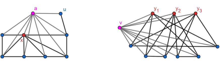
The Figure 5 shows the graphs of \(\gamma_{iI}(G)=3\). In the first graph, the vertex \(a\) is \(K_1\), the vertex \(x\) is of degree \(n-2\), which is not adjacent only to \(u\). In the second graph, the vertex \(v\) is \(K_1\) and \(\{y_1,y_2,y_3\}\) forms the \(\gamma_2\) – set \(S\).
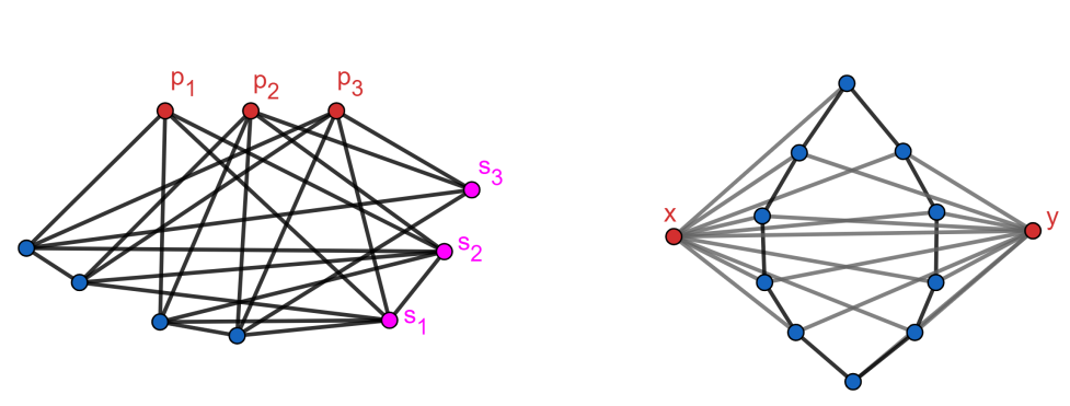
The Figure 6 shows the graphs of graphs of \(\gamma_{iI}(G)=3\). In the first graph, \(\{p_1,p_2,p_3\}\) forms the \(\gamma_2\) – set \(S\) and \(\{s_1,s_2,s_3\}\) forms the \(\gamma_2\) – set \(R\) in \(V-S\). In the second graph, \(x,y\) are the vertices of degree \(n-2\) with \(N(x) \neq N(y)\). ◻
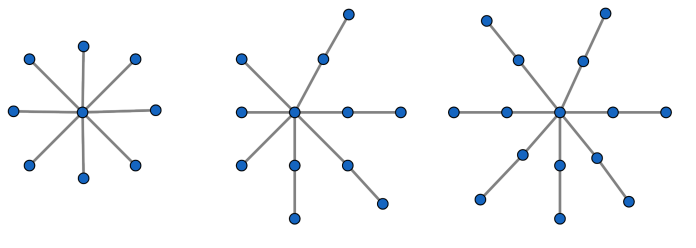
A wounded spider is a graph obtained by subdividing at most \(n-2\) edges of a star \(K_{1,n-1}\). A healthy spider is obtained by subdividing all the edges of a star. Let \(d_{T}(u)\) be the degree of \(u\) in the tree \(T\). Let \(T_v\) be the maximal subtree containing \(v\) and its descendants.
Theorem 4.1. For any tree \(T\) of order \(n \geq 3\),
\(\gamma_{iI}(T) \leq n-1\).
Proof. We prove this by induction hypothesis on \(n\), the number of vertices of \(T\). We can observe that \(diam(T) \geq 2\) since \(n \geq 3\) . When \(diam(T)=2\), then \(T\) has to be a star, which implies \(\gamma_{iI}(T)=n-1\). When \(diam(T)=3\), then \(T\) has to be a double star which implies \(\gamma_{iI}(T) \leq n-1\). Hence, we consider \(diam (T) \geq 4\) implying \(n \geq 5\). By induction hypothesis, there exists a \(\gamma_{iI}\) – function \(h^{'}\) for any subtree \(T^{'}\) of order \(m\) where \(3 \leq m < n\) having the property \(\gamma_{iI}(T^{'})=w(h^{'}) \leq m-1\). Consider a diametrical path \(\left(u_1, u_2,\ldots,u_k\right), (k \geq 5)\) of \(T\), so that the degree of \(u_2\) is maximum possible in \(T\). Let \(T_v\) be the maximal subtree containing \(v\) and its descendants. Let \(u_k\) be the root of \(T\) and proceed to the cases that follow.
Case 1. When \(d_{T}(u_2)\geq 3\).
Consider the case \(d_{T}(u_2)\geq 3\). Let \(T^{'}\) be the subtree with \(m\) vertices obtained by deleting \(u_2\) and its leaves from \(T\). By mathematical induction, the result holds for \(T^{'}\) and hence there is a \(\gamma_{iI}\) – function \(h^{'}\) on \(V(T^{'})\) such that \(w(h^{'})=\gamma_{iI}(T^{'}) \leq m-1\). Since \(u_2\) is a support vertex with \(l \geq 3\) leaf neighbors, there exists a \(\gamma_{I}\) – function on \(T^{'}\) which assigns \(2\) to \(u_2\) and \(0\) to its leaf neighbours.
We can define an IIDF \(f^{'}\)
on \(V(T)\) such that, it assigns \(1\) to its \(l\) leaf neighbours, \(f^{'}(u_2)=0\) , and \(f^{'}(x)=h^{'}(x)\) for all \(x \in V(T^{'})\). Hence \(\gamma_{iI}(T) \leq w(f^{'}) =
w(h{'})+l\) which implies, \(\gamma_{iI}(T) \leq (m-1) +l \leq n-(l+1)-1+l =
n-2 < n-1\).
In this case, we proved that \(\gamma_{iI}(T)
< n-1\).
Case 2. When \(d_{T}(u_2)=d_{T}(u_3)=2\).
Let a tree \(T^{'}\) of order
\(m\) be obtained by deleting \(u_1,u_2\) and \(u_3\). We have assumed that \(diam (T) \geq 4\) implying \(n \geq 5\) hence \(m \geq 2\). If \(m=2\), then \(T=P_5\) which implies, \(\gamma_{iI}(T)=4=n-1\). So, let us assume
that \(m \geq 3\). By the induction
hypothesis, there is a \(\gamma_{iI}\)
– function \(h^{'}\) on \(V(T^{'})\) such that \(w(h^{'})=\gamma_{iI}(T^{'}) \leq
m-1\). There exists a \(\gamma_{I}\) – function \(f\) on \(V(T)\) such that, \(f(u_2)=2\) and \(f(u_1)=f(u_3)=0\). We can define an IIDF
\(f^{'}\) on \(V(T)\) such that, \(f^{'}(u_2)=0\), \(f^{'}(u_1)=f^{'}(u_3)=1\) and \(f^{'}(x)=h^{'}(x)\) for all \(x \in V(T^{'})\). Hence \(\gamma_{iI}(T) \leq w(f^{'}) =
w(h{'})+2\) which implies, \(\gamma_{iI}(T) \leq (m-1) +2 \leq n-2 <
n-1\).
In this case, we proved that \(\gamma_{iI}(T)
< n-1\).
Case 3. When \(d_{T}(u_2)=2\) and \(d_{T}(u_3)\geq 3\).
The vertex \(u_2\) in the diametrical path is chosen such that, every child of \(u_3\) is a vertex similar to \(u_2\) or it is a leaf.
Subcase 3.1. When the vertex \(u_4\) is a support vertex with \(deg(u_4)=2\).
If \(u_4\) is a support vertex and \(deg(u_4)=2\), then \(T\) is a wounded spider or a healthy spider where \(q \geq 2\) edges of a star are subdivided.
i) Suppose \(u_3\) has no leaf as neighbours.
In this case \(T\) is a healthy spider. There exists an IDF \(f\) on \(V(T)\) which assigns \(1\) to \(u_3\) and to all vertices at a distance \(2\) from \(u_3\) and \(0\) to the rest of the vertices. The only possible IIDF \(f^{'}\) of \(f\) is defined such that \(f^{'}(u)=2\) if \(u\) is at a distance \(1\) from \(u_3\) and \(0\) to the rest of the vertices. Then we have \(\gamma_{iI}(T)= w(f^{'})=2q=\frac{2(n-1)}{2}=n-1\).
ii) Suppose \(u_3\) has \(l\) -leaves as neighbours.
In this case \(T\) is a wounded spider. There exists an IDF \(f\) on \(V(T)\) which assigns \(2\) to \(u_3\), \(1\) to all vertices at a distance \(2\) from \(u_3\) and \(0\) to the remaining vertices. The only possible IIDF \(f^{'}\) of \(f\) is defined such that it assigns \(1\) to the leaf neighbours of \(u_3\) and \(2\) to the remaining neighbours of \(u_3\). All the rest of the vertices of \(T\) will be assigned \(0\) under \(f^{'}\). Then \(\gamma_{iI}(T)= w(f^{'})\) and \(w(f^{'})=2q+l=\frac{2(n-l-1)}{2}+l=n-1\).
In Subcase 3.1, we proved that \(\gamma_{iI}(T)= n-1\).
Subcase 3.2. When the vertex \(u_4\) is not a support vertex of degree 2.
Let \(deg(u_4)\neq 2\) and let \(u_4\) is not a support vertex of \(T\). Suppose \(T^{'}=T-V(T_{{u}_{3}})\) and \(m \geq 3\). By induction hypothesis, there exists an IIDF \(h^{'}\) on \(V(T^{'})\) such that \(\gamma_{iI}(T^{'})= w(h^{'}) \leq m-1\). We observe that \(T_{u_{3}}\) is obtained by subdividing \(q \geq 1\) edges of a star.
i) Suppose \(u_3\) has no leaf as neighbours.
In this case, \(T_{u_{3}}\) is a
healthy spider. There exists an IDF \(f\) on \(V(T)\) which assigns \(1\) to \(u_3\) and to every grandchild of \(u_3\) and \(0\) to every child of \(u_3\). We can define an IIDF \(f^{'}\) of \(f\) where \(f^{'}(x)=h^{'}(x)\) for all \(x \in V(T^{'})\), it assigns \(2\) to every child of \(u_3\) and \(0\) to the rest of the vertices. This
implies,
\(\gamma_{iI}(T) \leq w(h^{'}) + 2q \leq
m -1 +2q \leq (n-2q-1) -1 +2q = n-2 < n-1.\)
ii) Suppose \(u_3\) has \(l\) -leaves as neighbours.
In this case \(T_{u_{3}}\) is a wounded spider. There exists an IDF \(f\) on \(V(T)\) which assigns \(2\) to \(u_3\) and \(1\) to every grandchild of \(u_3\) and \(0\) to every child of \(u_3\). We can define an IIDF \(f^{'}\) of \(f\) where \(f^{'}(x)=h^{'}(x)\) for all \(x \in V(T^{'})\), it assigns \(1\) to every leaf neighbour of \(u_3\) and \(2\) to the remaining neighbours of \(u_3\) and \(0\) to the rest of the vertices. This implies, \[\gamma_{iI}(T) \leq w(h^{'}) + 2q + l \leq m -1 +2q +l = (n-2q-l-1) -1 +2q+l = n-2 < n-1.\]
In Subcase 3.2, we proved that \(\gamma_{iI}(T) < n-1\). This proves the upper bound. ◻
Theorem 4.2. For any tree \(T\) of order \(n \geq 3\), \(\gamma_{iI}(T)= n-1\) if and only if \(T\) is a star, a wounded spider or a healthy spider.
Proof. Consider a tree with \(\gamma_{iI}(T)=n-1\). In the Theorem 4.1, we have proved that \(\gamma_{iI}(T) \leq n-1\). From the proof of the theorem 4.1, we can observe that, it attains equality only when \(T\) is a star, \(T=P_4\), \(T=P_5\) and \(T\) as in Subcase 3.1. All these trees are either stars, wounded spiders or healthy spiders.
Conversely, let \(T\) be a tree which is a star, a healthy spider or a wounded spider with its \(q\geq 0\) edges subdivided. Let \(v\) be the vertex of maximum degree in \(T\).
(i) If \(T\) is a star, then \(\gamma_{iI}(T)=n-1\).
(ii) If \(T\) is a healthy spider, then the only \(\gamma_{I}\) – function, \(f\) assigns \(1\) to \(v\) and all vertices at a distance \(2\) from it. The only \(\gamma_{iI}\) – function, \(f^{'}\) assigns \(2\) to all vertices at a distance \(1\) from \(v\) and \(0\) to the remaining vertices. Hence \(\gamma_{iI}(T)=n-1\).
(iii) If \(T\) is a wounded spider, then \(1 \leq q \leq n-2\). Let \(v\) have \(l \geq 1\) leaves as neighbors. A \(\gamma_{I}\) – function, \(f\) assigns \(2\) to \(v\) and \(1\) to all vertices at a distance \(2\) from it and \(0\) to the rest of the vertices. The IIDF, \(f^{'}\) assigns \(0\) to \(v\) and all vertices at a distance \(2\) from it. All leaves of \(v\) are assigned \(1\) and the rest of the neighbors of \(v\) can be assigned \(2\) under the function \(f^{'}\). Hence \(\gamma_{iI}(T)=2q+l = 2 (\frac{n-l-1}{2})+l=n-1\). ◻
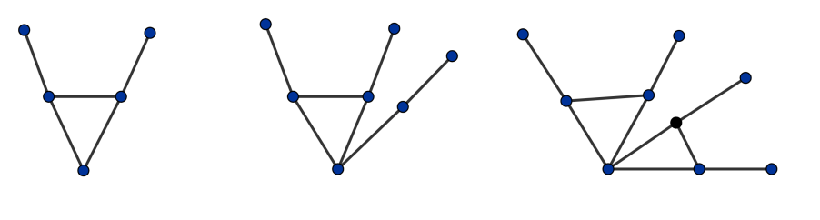
A graph having two non-adjacent pendant edges attached to \(C_3\) is called a bull graph, denoted by \(B\). We define a family G of connected graphs, which includes the graphs \(C_5\) and \(\mathcal{G}(t,r,s,m)\).
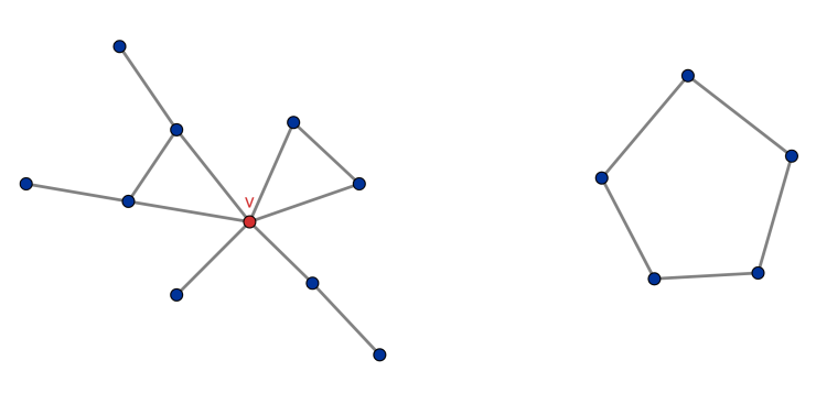
Graph \(\mathcal{G}(t,r,s,m)\): In this graph we can have \(t\geq 0\) number of \(P_2\), \(r\geq 0\) number of \(P_3\), \(s\geq 0\) number of \(C_3\), \(m\geq 0\) number of Bull graphs \(B\), where one vertex from each graph is identified/merged into a single vertex \(v\). From Bull graph \(B\) we select the vertex of degree \(2\) and from \(P_3\) we select the vertex of degree \(1\) to identify with vertex \(v\). Bull graph is a graph \(C_3\) having two non-adjacent pendant edges. Figure 8 depicts the graph \(\mathcal{G}(1,1,1,1)\) and \(C_5\) of graph family \(\mathcal{G}\). Few graphs are excluded from the graph family \(\mathcal{G}(t,r,s,m)\). They are \(\mathcal{G}(0,0,0,1),\) \(\mathcal{G}(0,0,0,2),\) \(\mathcal{G}(0,1,0,1)\) which are shown in Figure 8.
Theorem 5.1. For a connected graph \(G\) of order \(n \geq 3\),
\(\gamma_{iI}(G) \leq n-1\).
Proof. Consider a graph \(G\), which is connected and has \(n\geq 3\) vertices. If we remove any edge of \(G\), then its \(\gamma_{iI}(G)\) will either increase or remain the same but never decrease. Therefore, \(\gamma_{iI}(G) \leq \gamma_{iI}(T)\) for any spanning tree \(T\) of \(G\). Hence, by Theorem 4.1, we have \(\gamma_{iI}(G) \leq \gamma_{iI}(T) \leq n-1\). ◻
Theorem 5.2. For a connected graph \(G\) of any order \(n \geq 3\), \(\gamma_{iI}(G) = n-1\) if and only if \(G \in \mathcal{G}\).
Proof. Consider \(G\) which is connected and \(\gamma_{iI}(G)= n-1\). If \(T\) is any spanning tree of \(G\), then \(\gamma_{iI}(T)= n-1\), because deletion of edges will not decrease the \(\gamma_{iI}(G)\) and it cannot increase since it is the maximum. By Theorem 4.2, \(T\) is a star, a wounded spider or a healthy spider. So \(G\) is a super graph of \(T\) having \(T\) as a spanning tree. By adding all possible types of edges to \(T\), the \(\gamma_{iI}(G)\) will not decrease, and we can consequently derive the family \(\mathcal{G}\).
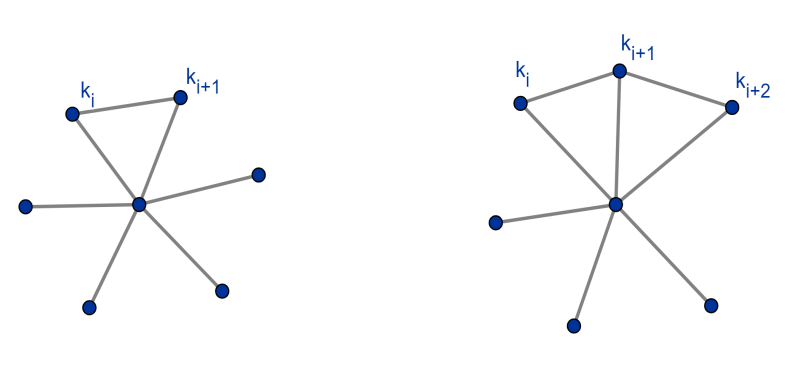
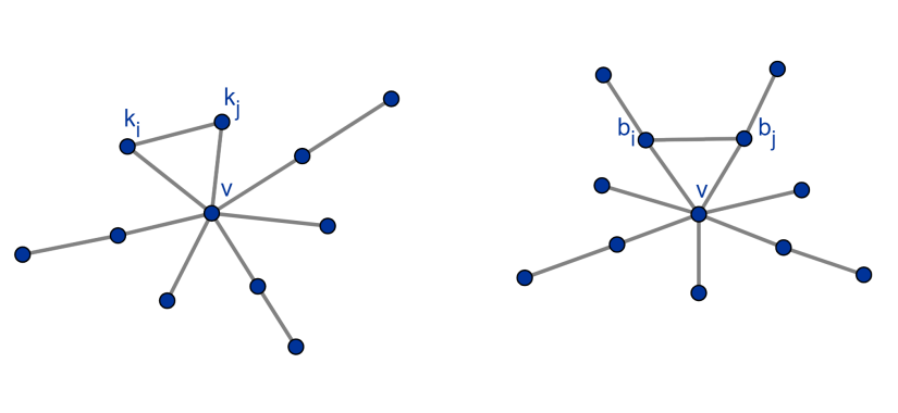
i) Let \(T\) be a star and \(k_1,k_2,\ldots,k_{n-1}\) be the leaves of \(T\). We add all possible types of edges to \(T\) so that its \(\gamma_{iI}(G)\) remains the same. If we add the edge \(k_i k_{i+1}\) to \(T\), then it results in \(\mathcal{G}(n-3,0,1,0)\) which has \(\gamma_{iI}(G)\) equals \(n-1\). If we add the edges \(k_i k_{i+1}\) and \(k_{i+1} k_{i+2}\), the resulted graph will have \(\gamma_{iI}(G)\) less than \(n-1\) as it has \(C_4\) as its subgraph. Figure 10 shows these graphs. Hence the only possible graphs of \(\gamma_{iI}(G)\) equal to \(n-1\) are \(\mathcal{G}(t,0,s,0)\) and \(\mathcal{G}(0,0,s,0)\) .
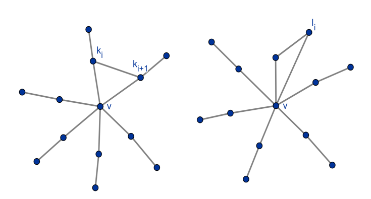
ii) Let \(T\) be a healthy spider. Let \(v\) be the vertex of maximum degree and \(k_1, k_2,\ldots,k_p\) be the adjacent vertices of \(v\). Let \(l_1, l_2,\ldots,l_p\) be the vertices of degree \(1\). If we add the edge \(k_i k_{i+1}\) to \(T\), then it results in \(\mathcal{G}(0,p-2,0,1)\) which has \(\gamma_{iI}(G)\) equals \(n-1\). If we add the edge \(l_i v\) to \(T\), then it results in \(\mathcal{G}(0,p-1,1,0)\) which has \(\gamma_{iI}(G)\) equals \(n-1\). Figure 11 shows these graphs.
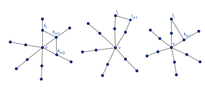
If we add the edges \(k_i k_{i+1}\) and \(k_{i+1} k_{i+2}\), the resulted graph will have \(\gamma_{iI}(G)\) less than \(n-1\) as it has \(C_4\) as its subgraph. Moreover, adding the edges \(l_i l_{i+1}\) or \(l_i k_{i+1}\) also will decrease the \(\gamma_{iI}(G)\). Figure 12 shows these graphs. Hence, the only possible graphs that can have \(\gamma_{iI}(G)\) equal to \(n-1\) are \(\mathcal{G}(0,r,s,m)\) where \(r\geq 0, s \geq 0, m\geq 0\). Furthermore, \(\mathcal{G}(0,0,0,1)\) , \(\mathcal{G}(0,0,0,2)\) and \(\mathcal{G}(0,1,0,1)\) are excluded as they have \(\gamma_{iI}(G)\) less than \(n-1\).
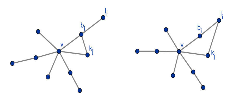
iii) Let \(T\) be a wounded spider. Let \(v\) be the vertex of maximum degree, \(b_1, b_2,\ldots,b_p\) be the vertices of degree \(2\) and \(l_i\) be the leaves adjacent to \(b_i\). Let \(k_1, k_2,\ldots,k_q\) be the leaves adjacent to \(v\). We omit the cases, which have already been discussed. Adding the edges \(k_i k_j\) or \(b_i b_j\) will keep the \(\gamma_{iI}(G)\) same which is shown in Figure 14.
Adding the edge \(b_i k_j\) decreases the \(\gamma_{iI}(G)\), when the degree of \(v\) is more than \(2\). When the degree of \(v\) is equal to \(2\), we get the graph \(\mathcal{G}(1,0,1,0)\) which is discussed in Case 1. Adding the edge \(l_i k_j\) also decreases the \(\gamma_{iI}(G)\) as it has \(C_4\) as its subgraph. This is shown in Figure 13. Hence, the only possible graphs that can have \(\gamma_{iI}(G)\) equal to \(n-1\) are \(\mathcal{G}(t,r,s,m)\) where \(t \geq 0, r\geq 0, s \geq 0, m\geq 0\).
Conversely, let \(G \in \mathcal{G}\). The only possible \(\gamma_{I}\) – function \(f\) to the graph \(\mathcal{G}(t,r,s,m)\) assigns \(2\) to \(v\) and \(0\) to all vertices adjacent to \(v\). Rest of the vertices are assigned \(1\) under \(f\). A \(\gamma_{iI}\) – function \(f^{'}\) is defined in such a way that, all vertices \(u\) with \(f(u)>0\) are assigned \(f^{'}(u)=0\). All the vertices adjacent to \(v\) and belonging to \(B\) or \(P_3\) are assigned \(2\) and the remaining vertices are assigned \(1\) under \(f^{'}\). This gives \(\gamma_{iI}(\mathcal{G}(t,r,s,m))=n-1\). From Proposition 2.1, \(\gamma_{iI}(C_5)=4=n-1\). ◻
Proposition 6.1. For every graph \(G\),
\(\gamma(G) \leq \gamma_{I}(G) \leq \gamma_{iI}(G),\)
and the upper bound is sharp for \(K_n\) with \(n\geq 2.\)
Proof. For any graph \(G\), a minimum dominating set or \(\gamma\) – set is always the subset of some \(\gamma_I\) – set. As a result \(\gamma(G) \leq \gamma_{I}(G)\). An IIDF is also an IDF. Hence \(\gamma_{I}(G) \leq \gamma_{iI}(G)\). For \(G\cong K_n\), we have \(\gamma_{I}(G) = \gamma_{iI}(G)\). ◻
Proposition 6.2. [2] For any graph \(G\) of order \(n\),
\(\gamma(G) \leq \gamma_{I}(G) \leq 2 \gamma(G).\)
Proposition 6.3. For every graph \(G\) of order \(n\),
\(\gamma_{i}(G) \leq \gamma_{iI}(G) \leq 2 \gamma_{i}(G)\).
Theorem 6.4. For every graph \(G\) of order \(n\geq 2\),
\(\gamma_{I}(G)+ \gamma_{iI}(G) \leq 2n,\)
and this bound is sharp for \(K_2\).
Proof. Let \(f=(V_0,V_1,V_2)\) be any \(\gamma_I\) – function and let \(f^{'}=(V^{'}_0,V^{'}_1,V^{'}_2)\) be any \(\gamma_{iI}\) – function. Every vertex \(v_i \in (V_1 \cup V_2)\) under \(\gamma_I\) – function, will be in \(V^{'}_0\) under \(\gamma_{iI}\) – function. Hence, \(f(v_i)+f^{'}(v_i) \leq 2\) for all \(1 \leq i \leq n\), which implies \(\sum_{i=1}^{n}\left(f(v_i)+f^{'}(v_i)\right) \leq 2n.\) This proves that, \(\gamma_{I}(G)+ \gamma_{iI}(G)\leq 2n.\) For \(K_2\), this sum is \(4=2n.\) ◻
Theorem 6.5. [11] If \(G\) is any connected graph of order \(n\geq 3\), then
\(\gamma_I(G) \leq \dfrac{3n}{4}\).
Theorem 6.6. For every connected graph \(G\) of order \(n\geq 3\),
\(\gamma_I(G) +\gamma_{iI}(G) \leq \dfrac{7n}{4}-1,\)
and it is a sharp bound for \(P_4\).
Proof. Let \(G\) be a connected graph \(G\) with \(n\geq 3\). By Theorem 6.5 we have, \(\gamma_I(G) \leq \dfrac{3n}{4}\). By adding this inequality to the inequality given in the Theorem 5.1, we arrive at, \(\gamma_I(G) +\gamma_{iI}(G) \leq \dfrac{3n}{4}+n-1 \leq \dfrac{7n}{4}-1\). The equality holds for \(P_4\) where \(\gamma_I(G) +\gamma_{iI}(G)=3+3=6=\dfrac{7n}{4}-1.\) ◻
Theorem 6.7. [7] If \(G\) is any graph, then
\(\gamma_{I}(G) \geq \dfrac{\gamma_{dR}(G)}{2}\).
Theorem 6.8. For every graph \(G\) of order \(n \geq 3\),
\(\gamma_{iI}(G) \leq \dfrac{7n}{4}-1-\dfrac{\gamma_{dR}(G)}{2}\).
Proof. Let \(G\) be a graph with \(n\geq 3.\) By Theorem 6.6 and Theorem 6.7, we have the required result. ◻
Theorem 6.9. [2] If \(G\) is any connected graph, then
\(\gamma_I(G) \geq \dfrac{2n}{\Delta(G)+2}\).
Theorem 6.10. For every connected graph \(G\) of order \(n \geq 3\),
\(\dfrac{2n}{\Delta(G)+2} \leq \gamma_{iI}(G) \leq \dfrac{7n}{4} -\dfrac{2n}{\Delta(G)+2} -1.\)
The upper bound is tight for \(C_4\) and the lower bound is tight for \(C_n\) when n is even.
Proof. Let \(G\) be a connected graph of order \(n\). By Theorem 6.6 and Theorem 6.7, we have the required upper bound. Since \(\gamma_I(G) \leq \gamma_{iI}(G)\), we get the lower bound. The lower bound is sharp for cycles \(C_n\) where \(n\) is even. When n is even, \(\gamma_{iI}(C_n)=\frac{n}{2}.\) The upper bound is sharp for \(C_4\) where \(\gamma_{iI}(C_4)=2.\) ◻
This field is expansive, offering endless opportunities for exploration. We propose a few open problems on the basis of our research.
Open problems
Characterize the graphs with \(\gamma_{I}(G)=\gamma_{iI}(G).\)
Characterize the graphs with \(\gamma_{iI}(G)=2\gamma_{i}(G).\)
Characterize the graphs with \(\gamma_I(G) +\gamma_{iI}(G) = \dfrac{7n}{4}-1\) for \(n\geq 3.\)
Characterize the graphs with \(\gamma_{I}(G)+\gamma_{iI}(G)=k \ \text{for any} \ k<\dfrac{7n}{4}-1\) for \(n\geq 3.\)
Explore the Nordhaus Gaddum inequalities for \(\gamma_{iI}(G).\)
Find bounds for \(\gamma_{iI}(G)\) in terms of different graph parameters for arbitrary graphs or some classes of graphs.
Characterize the graphs with \(\gamma_{iI}(G)=k\) for some \(k\) where \(4 \leq k \leq n-2.\)
Explore the relation between \(\gamma_{idR}(G)\) and \(\gamma_{iI}(G)\) for graphs.
Explore the relation between \(\gamma_{iI}(G)\) and \(\gamma_{i}(G)\) for graphs.