
Let \(G=(V,E)\) be a graph with a (finite) set \(V=V(G)\) of vertices and a set \(E=E(G)\) of edges. The distance from vertex \(u\) to vertex \(v\) in \(G\), denoted by \(\mathop{\mathrm{dist}}_G(u,v)\), is the length of a shortest path from \(u\) to \(v\). So, the diameter \(d=\mathop{\mathrm{diam}}(G)\) is the furthest distance between any pair of vertices in \(G\). If \(G\) has \(n\) vertices, its distance matrix \(\mbox{ $D$}\) is an \(n\times n\) matrix with entries \((\mbox{ $D$})_{u,v}=\mathop{\mathrm{dist}}_G(u,v)\). This matrix has been extensively studied in the literature and has interesting applications, both theoretical and practical (for instance, in telecommunication, chemistry, etc.); see Edelberg, Garey, and Graham [7], and Dededzi [6]. The results in the following theorem, which we use in this paper, are due to Graham and Pollak [11], and Bapat, Kirkland, and Neumann [3].
Theorem 1.1. Let \(G\) be a graph with distance matrix \(\mbox{ $D$}(G)\). Then, the following statements hold.
(i) If \(G=T\) is a tree, the determinant of \(\mbox{ $D$}(T)\) only depends on the number of its vertices \(n\): \(\det \mbox{ $D$}(T)=(-1)^{n-1}(n-1)2^{n-2}\) [11].
(ii) Let \(G\) be a unicyclic graph. Then, \(\det \mbox{ $D$}(G)=0\) when the only cycle of \(G\) has an even number of edges; and \(\det \mbox{ $D$}(G)=(-2)^m [k(k + 1) + \frac{2k+1}{2} m]\) if \(G\) has \(2k+1+m\) vertices and a cycle with \(2k+1\) edges [3].
A vertex subset \(C=\{z_1,z_2,\ldots,z_c\}\subset V\) is a resolving set if every vertex \(u\in V\) is uniquely determined by the vector \[\mbox{ $\rho$}=\mbox{ $\rho$}(u|C)=(\mathop{\mathrm{dist}}_G(u,z_1),\mathop{\mathrm{dist}}_G(u,z_2),\ldots,\mathop{\mathrm{dist}}_G(u,z_c)),\] which is called the representation (or position) of \(u\) with respect to \(C\). The metric dimension of \(G\), denoted by \(\dim(G)\), is the minimum cardinality of a resolving set. Notice that a vertex subset \(C\subset V\) is a resolving set of \(G\) if the \(|C|\times |V|\) submatrix of \(\mbox{ $D$}(G)\), with rows indexed by the vertices of \(C\), has all its columns different, and the metric dimension of \(G\) is the minimum cardinality of such a subset. The notion of metric dimension was introduced independently by Harary and Melter [13] and by Slater [18]. Since then, there has been extensive literature on the topic. For example, Cáceres, Hernando, Mora, Pelayo, Puertas, Seara, and Wood [4] studied the metric dimension of the Cartesian product \(G\Box H\) of graphs \(G\) and \(H\). As one of their main results, they provided a family of graphs \(G\) with bounded metric dimension for which the metric dimension of \(G\Box G\) is unbounded. Moreover, Bailey and Cameron [2] dealt with the metric dimension of the Johnson and the Kneser graphs. In particular, they computed the metric dimension of the former, which can be defined as the \(k\)-token graph of \(K_n\) (see the end of the following paragraph). In general, it is known that computing the metric dimension of a graph is an NP-hard problem; see Garey and Johnson [17, p. 204]. Some applications of the metric dimension approach are in network theory and combinatorial optimization; see Chartrand and Zhang [19] for a survey.
In this paper, we use a generalization of symmetric powers or token graphs, which we call supertoken graphs. Audenaert, Godsil, Royle, and Rudolph [1] defined the \(k\)-symmetric power of a graph \(G=(V,E)\), with vertices the \(k\)-subsets of \(V\), and two vertices are adjacent if their symmetric difference is the set of end-vertices of an edge in \(E\). Fabila-Monroy, Flores-Peñaloza, Huemer, Hurtado, Urrutia, and Wood [9] renamed them as the \(k\)-token graph of \(G\) and denoted it by \(F_k(G)\). The reason is that the vertices of \(F_k(G)\) correspond to the different placements of \(k\) tokens at the vertices where at most one token appears at each vertex, and two vertices are adjacent if one of the corresponding placements can be obtained from the other by moving one of its tokens to an unoccupied adjacent vertex.
The Laplacian spectra of token graphs were studied by Dalfó, Duque, Fabila-Monroy, Fiol, Huemer, Trujillo-Negrete, and Zaragoza Martínez [5]. As an important example of token graphs, we must mention that the Johnson graphs can be defined as \(J(n,k)=F_k(K_n)\) for any integers \(n\ge 2\) and \(1\le k<n\).
Let us consider the following model of communication. Given a set of \(n\) possible symbols corresponding to the vertices of a graph \(G\), we assume that instead of single symbols or (ordered) strings of them, we transmit multisets of \(k\) (not necessarily different) symbols. Moreover, we assume that the probability of error in each symbol is small enough to assume that, in the transmission of a multiset, at most one symbol is confused. In other words, the probability of two or more wrong symbols can be neglected. In this framework, the so-called confusability graph turns out to be a \(k\)-supertoken graph. This kind of token graph was introduced by Hammack and Smith [12], who named them reduced \(k\)-th power of graphs, and provided constructions of minimum cycle bases for them.
This paper is structured as follows. In the following section, we consider the construction and properties of two infinite families of graphs \(G(d,c)\) and \(G^+(d,c)\), which, in both cases, can be considered as graphs on alphabets. The latter allows us to provide a tight lower bound on its metric dimension. In Section 3, the definition of the supertoken graphs \({\cal F}_k(G)\) is given, and we find its metric properties when \(G\) is a complete graph \(K_n\) and a general graph. Finally, in Section 4, we establish an upper bound on the metric dimension of \({\cal F}_k(K_n)\), and \({\cal F}_k(G)\) for a general graph \(G\).
Generally, graphs on alphabets are constructed by labeling the vertices with words on a given alphabet and specifying rules that relate pairs of different words to define the edges, see Gómez, Fiol, and Yebra [10]. In this section, we construct two families of graphs on alphabets to obtain graphs with a maximum number of vertices for a given metric dimension.
The graphs in the following definition allow us to get a tight lower bound for the metric dimension.
Definition 2.1. Given integers \(d\) and \(c\), the graph \(G(d, c)\) has as its vertex set all sequences \(x = x_1x_2 \ldots x_c\) with \(x_i \in [1, d] = \{1, 2, \ldots, d\}\). (So \(G(d, c)\) has order \(dc\).) Moreover, two vertices \(x = x_1x_2 \ldots x_c\) and \(y = y_1y_2 \ldots y_c\) are adjacent if and only if \(|x_i – y_i| \in \{0, 1\}\) for every \(i =\{1, 2, \ldots, c\}\).
Note that the elements in the sequences describing the vertex labels need not be distinct.
The following result shows some basic metric properties of the graph \(G(d,c)\).
Lemma 2.2. Let \(x\) and \(y\) be two generic vertices of the graph \(G=G(d,c)\).
(i) If \(x=x_1x_2\ldots x_c\) and \(y=y_1y_2\ldots y_c\), the distance between \(x\) and \(y\) is \[\mathop{\mathrm{dist}}_G(x,y)=\max\limits_{i\in[1,c]}\{|x_i-y_i|\}.\] (ii) The eccentricity of the vertex \(x\) is \[\mathop{\mathrm{ecc}}_G(x)=\max\limits_{i\in[1,c]}\{x_i,d-x_i\}.\]
(iii) The diameter of the graph \(G(d,c)\) is \[\mathop{\mathrm{diam}}(G(d,c))=d-1.\]
Proof. (i) From the adjacency conditions in Definition 2.1, it is clear that \(\mathop{\mathrm{dist}}_G(x,y)=\max\limits_{i\in[1,c]}\{|x_i-y_i|\}\). To follow a shortest path from \(x\) to \(y\), note that each step \(x_i\) can be changed to \(x_i+1\) or \(x_i-1\) for every \(i=1,\ldots,c\). Thus, each \(x_i\) can be changed to \(y_i\) in exactly \(|x_i-y_i|\) steps and, hence, \(\mathop{\mathrm{dist}}(x,y)\) is as claimed.
(ii) By (i), every vertex \(y\) satisfies \(\mathop{\mathrm{dist}}_G(x,y)\le \max\limits_{i\in[1,c]}\{x_i,d-x_i\}\), and, for example, a vertex at maximum distance from \(x\) is either \(11\ldots 1\) or \(dd\ldots d\).
(iii) This is a consequence of (i) and (ii) since \(\max\limits_{i\in[1,c]}\{|x_i-y_i|\}=d-1\) and \(\min_{i\in[1,c]}\{x_i\}\geq1\). ◻
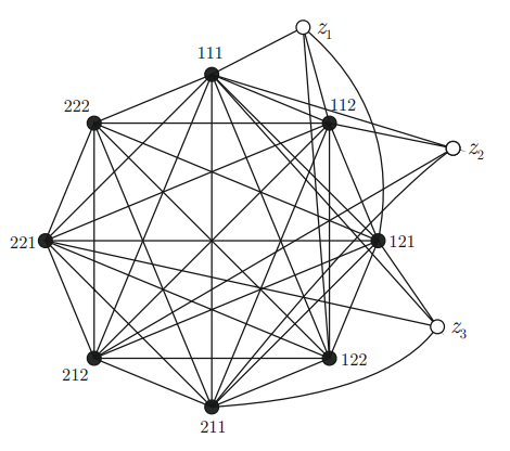
Definition 2.3. Given integers \(d\) and \(c\) with \(d\leq c\), the graph \(G^+(d,c)\) is obtained from \(G(d,c)\) by adding the vertices \(z_1,z_2,\ldots,z_c\) and, for every \(i=1,2,\ldots,c\), the vertices \(z_i\) are adjacent to all vertices \(x=x_1x_2\ldots x_c\) with \(x_i=1\).
Proposition 2.4. Let \(G=(V,E)\) be a graph with \(n\) vertices and diameter \(d\). Let \(c=c(d,n)\) be the minimum integer satisfying \(n\le d^c+c\). Then, the metric dimension of \(G\) satisfies \[\label{bound-dim} \dim(G)\ge c(d,n), \tag{1}\] and the bound is tight.
Note that this bound and its tightness were known; see the proof by Khuller, Raghavachari, and Rosenfeld [15], Theorem 3.6, and a generalization by Hernando, Mora, Pelayo, Seara, and Wood [14], Lemma 3.2.
As an example, we show the graph \(G^+(2,3)\) in Figure 1.
For some graphs, the inequality (1) can be improved. Let us show an example. A graph \(G=(V,E)\) with diameter \(d\) is distance-uniform if every vertex has the same number of vertices at distance \(i=1,\ldots,d\). That is, the numbers \(k_i(u)\), for \(i=0,1,\ldots,d\), do not depend on the vertex \(u\in V\), and we simply write \(k_i\). Some well-known examples of distance-uniform graphs are the vertex-transitive graphs and the distance-regular graphs. We call the sequence of numbers \(k_0(= 1), k_1, \ldots, k_d\) the distance-level sequence of a distance-uniform graph \(G = (V, E)\) of diameter \(d\). Then, the following result is straightforward.
Lemma 2.5. Let G be a distance-uniform graph of diameter \(d\), order \(n\) and distance-level sequence \(k_0(= 1), k_1,\) \(\ldots, k_d\). Let \(S(\mu; k_0, k_1, \ldots, k_d)\) be the set of sequences of length \(\mu\) having at most \(k_i\) numbers \(i\) with \(i \in [1, d]\). Then, \[n \leq |S(\mu; k_0, k_1, \ldots, k_d)|.\]
Here, we consider the k-supertoken graph \({\cal F}_k(G)\) defined as follows. Let \(G\) be a graph on \(n\) vertices. Then, for some integer \(k\ge 1\), each vertex of \({\cal F}_k(G)\) corresponds to \(k\) indistinguishable tokens placed in some of the (not necessarily distinct) \(n\) vertices in \(G\). Then, the vertex set of \({\cal F}_k(G)\) corresponds to the \(k\)-element multi-sets chosen from the \(n\)-element vertex set of \(G\), and its cardinality is given by \[%|CR^n_k|= {{n+k-1}\choose{k}} = {{n+k-1}\choose{n-1}}.\]
Thus, every vertex of \({\cal F}_k(G)\) corresponds to a way of placing \(k\) (indistinguishable) tokens in some of the \(n\) vertices, say \(1,2,\ldots,n\), of \(G\). For instance, \(11122455\in CR_8^5\) corresponds to having 3 tokens at vertex 1, 2 tokens at vertex 2, no token at vertex 3, 1 token at vertex 4, and 2 tokens at vertex 5, which we represent by the sequence \(32012\). In general, we represent each vertex \(\mbox{ $u$}\) of \({\cal F}_k(G)\) by a (non-negative) \(n\)-vector or \(n\)-sequence \[\mbox{ $u$}=(u_1,u_2,\ldots,u_n)\equiv u_1u_2\ldots u_n\quad \mbox{with } \sum\limits_{i=1}^{n}u_i=k.\]
Moreover, two of its vertices, \(\mbox{ $u$}\) and \(\mbox{ $v$}\), are adjacent if one token of the multiset representing \(\mbox{ $u$}\) is moved along an edge to another vertex (so obtaining the multiset representing \(\mbox{ $v$}\)). Then, notice that (the multisets of) \(\mbox{ $u$}\) and \(\mbox{ $v$}\) have \(k-1\) elements in common. Curiously enough, if \(P_n\) is the path graph on \(n\) vertices, it turns out that the \(2\)-supertoken graph \({\cal F}_2(P_n)\) is isomorphic to the 2-token graph \(F_2(P_{n+1})\). The isomorphism between the vertices of \({\cal F}_2(P_n)\) and \(F_2(P_{n+1})\) is given by the mapping \(ij\mapsto i(j+1)\).
The \(k\)-supertoken graphs were introduced by Hammack and Smith [12], who named them reduced \(k\)-th power of graphs, and provided constructions of minimum cycle bases for them.
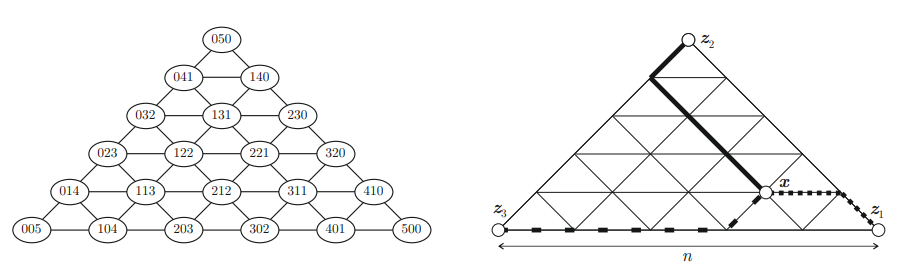
First, we consider the case of \(G=K_n\), the complete graph on \(n\) vertices. For example, \({\cal F}_5(K_3)\) is drawn in Figure 2 (left).
In the following result, we describe some basic metric properties of \({\cal F}_k(K_n)\).
Proposition 3.1. Given integers \(n\) and \(k\), the supertoken graphs \({\cal F}_k={\cal F}_k(K_n)\) satisfy the following statements.
(i) The distance between two generic vertices \(\mbox{ $x$}=x_1x_2\ldots x_n\) and \(\mbox{ $y$}=y_1y_2\ldots\) \(y_n\) is \[\mathop{\mathrm{dist}}_{{\cal F}_k}(\mbox{ $x$},\mbox{ $y$})=\frac{1}{2}\sum\limits_{i=1}^{n}|x_i-y_i|. \label{dist(x,y)} \tag{2}\]
(ii) The eccentricity of a vertex \(\mbox{ $x$}=x_1x_2\ldots x_n\) is \[\mathop{\mathrm{ecc}}_{{\cal F}_k}(\mbox{ $x$})=k-\min_{1\le i\le n}{x_i}. \label{ecc(x)} \tag{3}\]
(iii) The diameter of \({\cal F}_k(K_n)\) is \(\mathop{\mathrm{diam}}({\cal F}_k(K_n))=k\).
(iv) The radius of \({\cal F}_k(K_n)\) is \(\mathop{\mathrm{rad}}({\cal F}_k(K_n))=n-\lfloor \frac{n}{k}\rfloor\).
Proof. (i) Let us consider the sets \(X=\{i: x_i> y_i\}\), \(Y=\{i: x_i< y_i\}\), and \(Z=\{i: x_i=y_i\}\). Then, \[\begin{aligned} \sum\limits_{i\in X} (x_i-y_i) &=\sum\limits_{i\in X} x_i- \sum\limits_{i\in X} y_i=n-\sum\limits_{i\in Z} x_i-\sum\limits_{i\in Y} x_i-\left(n-\sum\limits_{i\in Z} y_i-\sum\limits_{i\in Y} y_i\right) \nonumber\\ &=\sum\limits_{i\in Y} (y_i-x_i).\label{equality} \end{aligned} \tag{4}\]
Then, to go from \(\mbox{ $x$}\) to \(\mbox{ $y$}\), in each step, we move a token from a vertex \(i\in X\) (so reducing the value of \(x_i\)) to a vertex \(j\in Y\) (increasing the value of \(y_j\)). Thus, the length of the path is \(\sum\limits_{i\in X}(x_i-y_i)\) and, from (4), \((i)\) follows.
(ii) Given the vertex \(\mbox{ $x$}=x_1x_2\ldots x_n\) with \(x_h=\min_{1\le i\le n} x_i\), the vertex \(\mbox{ $y$}=y_1y_2\ldots y_n\) is at maximum distance from \(\mbox{ $x$}\) when we have to move the maximum possible number of tokens, one at a time. That is, when \(y_j=0\) for \(j\neq h\) and \(y_h=k-x_h\).
(iii) According to (2), the maximum possible distance between two vertices \(\mbox{ $x$}\) and \(\mbox{ $y$}\) is \(k\). That is, when the \(\sum\limits_{i=1}^{n}|x_i-y_i|=2k\). Using the notation in the proof of \((i)\), this occurs when, for all \(i\in X\), \(\sum\limits_{i\in X}x_i=k\) and \(y_i=0\), (and, hence, for all \(j\in Y\), \(\sum\limits_{j\in Y}y_j=k\) and \(x_j=0\)).
(iv) From (3), the minimum eccentricity of a vertex \(\mbox{ $x$}\) is obtained when \(x_h=\min_{1\le i\le n}{x_i}\) is maximum. Since \(\sum\limits_{i=1}^n x_i=k\), this occurs when \(x_h=\lfloor k/n\rfloor\). ◻
Example 3.2. In the graph \({\cal F}={\cal F}_3(K_5)\) of Figure 2 (left), we get:
(i) \(\mathop{\mathrm{dist}}_{{\cal F}}(203,140)=\frac{1}{2}(1+4+3)=4\);
(ii) \(\mathop{\mathrm{ecc}}_{\cal F}(122)=5-\min\{1,2\}=4\);
(iii) \(\mathop{\mathrm{dist}}_{\cal F}(500,041)=\mathop{\mathrm{diam}}({\cal F})=5\);
(iv) \(\mathop{\mathrm{rad}}({\cal F}) =\mathop{\mathrm{ecc}}(122) = 5- \lfloor5/3\rfloor = 4\).
Let \(G=(V,E)\) be a (connected) graph with vertex set \(\{1,2,\ldots,n\}\). The metric properties in the following result are direct generalizations of Proposition 3.1.
Recall that an \(r\)-antipodal graph is a connected graph in which each vertex has exactly \(r\) vertices at maximum distance.
Proposition 3.3. Let \(G\) be a graph on \(n\) vertices, diameter \(d\), and radius \(r\). Given an integer \(k\), the supertoken graphs \({\cal F}_k(G)\) satisfy the following statements.
(i) The diameter of \({\cal F}_k(G)\) is \(\mathop{\mathrm{diam}}({\cal F}_k(G))=kd\).
(ii) The radius of \({\cal F}_k(G)\) is \(\mathop{\mathrm{rad}}({\cal F}_k(G))\le kr\).
(iii) If \(G\) is an \(r\)-antipodal graph with diameter \(d\), then \({\cal F}_k(G)\) has \(r\) vertices mutually at distance \(kd\).
Proof. (i) Let \(i,j\in V(G)\) such that \(\mathop{\mathrm{dist}}_G(i,j)=d\). Then, in \({\cal F}_k(G)\), to go from a vertex \(\mbox{ $x$}\) to vertex \(\mbox{ $y$}\) such that \(x_i=k\) (with \(x_h=0\) for \(h\neq i\)) and \(y_j=k\) (with \(y_h=0\) for \(h\neq j\)) corresponds to moving, in \(G\), \(k\) tokens from vertex \(i\) to vertex \(j\). Since the distance between \(i\) and \(j\) is \(d\) and we move \(k\) tokens, this requires exactly \(kd\) steps.
(ii) Let \(i\) be such that \(\mathop{\mathrm{ecc}}(i)=r\). Then, we claim that, in \({\cal F}_k(G)\), the eccentricity of a vertex \(\mbox{ $x$}\) such that \(x_i=k\) (with \(x_h=0\) for \(h\neq i\)) is at most \(kr\). Indeed, in \(G\), we can move every token at vertex \(i\) to any vertex \(j\) in at most \(r\) steps. This means that we can go, in \({\cal F}_k(G)\), from \(\mbox{ $x$}\) to any vertex \(\mbox{ $y$}\) in, at most, \(kr\) steps.
(iii) If \(i_1,i_2,\ldots,i_r\) are vertices in \(G\) at distance \(d\) from each other, the \(r\) vertices of \({\cal F}_k(G)\) \(\mbox{ $x$}_1,\mbox{ $x$}_2,\ldots,\mbox{ $x$}_r\) such that \((\mbox{ $x$}_1)_{i_1}=k\), \((\mbox{ $x$}_2)_{i_2}=k\), \(\ldots\), \((\mbox{ $x$}_r)_{i_r}=k\) are, from (i), mutually at distance \(kd\). ◻
Contrary to the case when \(G=K_n\), when \(G\) is a general graph, there is no closed formula for the distance between two vertices \(\mbox{ $x$}\) and \(\mbox{ $y$}\). Instead, we give the following algorithm to find a shortest path from \(\mbox{ $x$}\) to \(\mbox{ $y$}\) in \({\cal F}_k(G)\):
Algorithm 3.4. Finding the distance from a vertex \(\mbox{ $x$}=x_1\ldots x_n\) to a vertex \(\mbox{ $y$}=y_1\ldots y_n\) in \({\cal F}_k(G)\) for a given graph \(G\) and a positive integer \(k\).
(a) Given \(\mbox{ $x$}=x_1x_2\ldots x_n\) and \(\mbox{ $y$}=y_1y_2\ldots y_n\), let \(X=\{i:x_i>y_i\}\) and \(Y=\{j:y_j>x_j\}\). Thus, if \(x_h=y_h\) for some \(h\in[1,n]\), such index \(h\) is neither present in \(X\) nor in \(Y\).
(b) Consider the vectors
\(\mbox{ $x$}'=(i_1^{x_{i_1}-y_{i_1}},i_2^{x_{i_2}-y_{i_2}},\ldots,i_{\sigma}^{x_{i_{\sigma}}-y_{i_{\sigma}}})\) such that \(i_{\ell}\in X\) for \(\ell=1,\ldots,\sigma\), and \(i_{\ell}^{x_{i_{\ell}}-y_{i_{\ell}}}\) represents a sequence of length \(x_{i_{\ell}}-y_{i_{\ell}}\), where each term in the sequence is \(i_{\ell}\).
\(\mbox{ $y$}'=(j_1^{y_{j_1}-x_{j_1}},j_2^{y_{j_2}-x_{j_2}},\ldots,j_{\sigma}^{y_{j_{\tau}}-x_{j_{\tau}}})\) such that \(j_h\in Y\) for \(h=1,\ldots,\tau\), and \(j_h^{y_{j_h}-x_{j_h}}\) stands for \(\displaystyle \underbrace{j_h,\ldots,j_h}_{y_{j_h} – x_{j_h}}\).
(Notice that \(\mbox{ $x$}'\) and \(\mbox{ $y$}'\) can also be seen as multisets with the same number, say \(n'=\sum\limits_{i_{\ell}\in X}(x_{i_{\ell}}-y_{i_{\ell}})=\sum\limits_{j_h\in Y}(y_{i_h}-x_{i_h})\), of vertices in \(G\)).
(c) Define a distance \(n'\times n'\) matrix \(\mbox{ $D$}\) with rows and columns indexed by the entries of \(\mbox{ $x$}'\) and \(\mbox{ $y$}'\) respectively, and entries \((\mbox{ $D$})_{i_{\ell} j_h}=\mathop{\mathrm{dist}}_G(i_{\ell}, j_h)\). (This matrix represents a weighted complete bipartite graph \(K^*_{n',n'}\), where the edge \(\{i_{\ell},j_h\}\) has weight \(\mathop{\mathrm{dist}}_G(i_{\ell},j_h)\)).
(d) Apply the known algorithm to find a minimum weighted perfect matching in \(K^*_{n',n'}\). This algorithm, usually called the ‘Hungarian method’, is known to be ‘strongly polynomial’; that is, it is polynomial in the number of weights (distances) used. See, for instance, Edmonds [8] and Kuhn [16].
(e) For each pair \(i_{\ell}\) and \(j_h\) of paired vertices of the matching, we move in \(G\) a token from \(i_{\ell}\) to \(j_h\). (Since in \(K^*_{n',n'}\) there are possibly vertices with the same labels, the above operation may need to be repeated several times).
Example 3.5. Let \({\cal{F}}_9(G)\) with \(G=C_6\) is the cycle graph with vertex set
\(\{1,2,\ldots,6\}\). Let us consider
the vertices \(\mbox{
$x$}=310212\) and \(\mbox{
$y$}=201132\) of \({\cal{F}}_9(G)\). Then, since we only need
to move the tokens that do not coincide between \(\mbox{ $x$}\) and \(\mbox{ $y$}\), \(X=\{1,2,4\}\), \(Y=\{3,5\}\), \(\mbox{ $x$}'=(1,2,4)\), \(\mbox{
$y$}'=(3,5^2)=(3,5,5)\). The distance matrix between the
entries (vertices in \(G\)) of \(\mbox{ $x$}'\) and \(\mbox{ $y$}'\) is
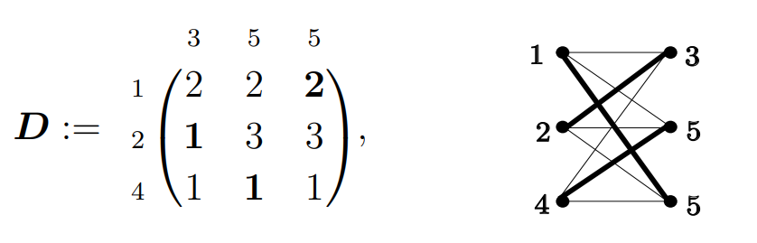
Notice that the minimization of the sum of the weights in \(\mbox{ $D$}\) (or distances in \(G\)) ensures that this algorithm gives a shortest path.
For a specific resolving set of \({\cal F}_k(G)\), the position of a vertex \(\mbox{ $x$}\) is easily computed. Indeed, consider the distance between a generic vertex \(\mbox{ $x$}=x_1x_2\ldots x_n\) and the vertex \(\mbox{ $y$}=0\ldots0k0\ldots0\), where the \(k\) is the \(j\)-th entry for some \(1\le j\le n\). Then, \[\mbox{ $x$}'=(1^{x_1},\ldots,(j-1)^{x_{j-1}}, (j+1)^{x_{j+1}},\ldots, n^{x_n})\quad\mbox{and}\quad \mbox{ $y$}'=(j^{\ell}-x_{j}).\]
Then, the distance matrix \(\mbox{ $D$}\) in point 3 of the algorithm has dimensions \(({\ell}-x_{j})\times ({\ell}-x_{j})\) with \(\ell-x_i\) columns indexed by \(j\), and all its rows equal to \[(\mathop{\mathrm{dist}}(1,j)^{x_1},\ldots,\mathop{\mathrm{dist}}(j-1,j)^{x_{j-1}},\mathop{\mathrm{dist}}(j+1,j)^{x_{j+1}},\ldots, \mathop{\mathrm{dist}}(n,j)^{x_n}).\]
Thus, we can pair \(1\) with \(j\) \(x_1\) times, \(2\) with \(j\) \(x_2\) times, etc. In other words, seen in \(G\), we move \(x_1\) tokens from 1 to \(j\) (with a total number of steps \(x_1\mathop{\mathrm{dist}}(1,j)\)), \(x_2\) tokens from \(2\) to \(j\) (with a total number of steps \(x_2\mathop{\mathrm{dist}}(2,j)\)), etc. Putting all together, to go from vertex \(\mbox{ $x$}\) to \(\mbox{ $y$}\) in \({\cal F}_k(G)\) requires \(x_i\mathop{\mathrm{dist}}_G(i,j)\) steps for every \(i=1,2,\ldots,n\). Thus, we have proved the following result.
Lemma 3.6. Given the supertoken graph \({\cal F}_k={\cal F}_k(G)\) of the graph \(G=(V,E)\) with vertex set \(V=\{1,2,\ldots,n\}\), let us consider the subset of \(V({\cal F}_k)\) \[C=\{\mbox{ $z$}_1,\mbox{ $z$}_2,\ldots,\mbox{ $z$}_n\}=\{k0\ldots0,\ 0k0\ldots0,\ \ldots,\ 0\ldots0k\}. \label{resolv} \tag{5}\]
Then, the distance between a vertex \(\mbox{ $x$}=x_1x_2\ldots x_n\in V({\cal F}_k)\) and the vertex \(\mbox{ $z$}_j\) is \[\mathop{\mathrm{dist}}_{{\cal F}_k}(\mbox{ $x$},\mbox{ $z$}_j)=\sum\limits_{i=1}^n x_i\mathop{\mathrm{dist}}_G(i,j). \tag{6}\]
Corollary 3.7. Let \(G\) be a graph on \(n\) vertices, with diameter \(d\) and distance matrix \(\mbox{ $D$}\). Let \(C\) be the vertex subset of \({\cal F}_k={\cal F}_k(G)\) in Lemma 3.6. Then, the position \(\mbox{ $\rho$}\) of a vertex \(\mbox{ $x$}=(x_1,x_2,\ldots,x_n)\in V({\cal F}_k)\) (represented as a vector) with respect to \(C\) is \[\mbox{ $\rho$}=\mbox{ $\rho$}(\mbox{ $x$}|C)=\mbox{ $x$}\mbox{ $D$}. \tag{7}\]
Proof. Just notice that, for every \(j=1,2,\ldots,n\), \[(\mbox{ $x$}\mbox{ $D$})_j=\sum\limits_{i=1}^nx_i(\mbox{ $D$})_{ij}=\sum\limits_{i=1}^nx_i\mathop{\mathrm{dist}}_G(i,j)=\mathop{\mathrm{dist}}_{{\cal F}_k}(\mbox{ $x$},\mbox{ $z$}_j)=\rho_j,\] where we used the definition of \(\mbox{ $D$}\) and Lemma 3.6. ◻
The above results suggest the following definition.
Definition 3.8. Given a graph \(G\) on \(n\) vertices and an integer \(k\ge 1\), we say that a non-negative vector \(\mbox{ $\rho$}=(\rho_1,\rho_2,\ldots,\rho_n)\) is \((G,k)\)-feasible if there exists a vertex \(\mbox{ $x$}\) of \({\cal F}_k(G)\) whose position with respect to the set \(C\) in (5) is \(\mbox{ $\rho$}\).
For a nonsingular matrix \(\mbox{ $D$}\), we have the following characterization of feasible vectors.
Lemma 3.9. Let \(G\) have a nonsingular distance matrix \(\mbox{ $D$}\). Then, a vector \(\mbox{ $\rho$}\) is \((G,k)\)-feasible for some \(k\) if and only if \(\mbox{ $x$}=\mbox{ $\rho$}\mbox{ $D$}^{-1}\) is a non-negative integer vector whose components sum up to \(k\).
Proof. Clearly, the vector \(\mbox{ $x$}\) so obtained represents a vertex of the supertoken graph \({\cal F}_k(G)\) if and only if it satisfies the conditions. Moreover, its position with respect to \(C\) is \(\mbox{ $x$}\mbox{ $D$}=\mbox{ $\rho$}\mbox{ $D$}^{-1}\mbox{ $D$}=\mbox{ $\rho$}\), as required. ◻
Example 3.10. The distance matrix of the complete graph \(K_n\) coincides with its adjacency matrix \(\mbox{ $D$}=\mbox{ $A$}=\mathop{\mathrm{circ}}(0,1,1,\ldots,1)\), with inverse \(\mbox{ $D$}^{-1}=\frac{1}{n-1}\mathop{\mathrm{circ}}(2-n,1,1,\ldots,1)\). Then, in the graph \({\cal F}_3(K_5)\) of Figure 2 (left), we show that the vector \(\mbox{ $\rho$}=(2,4,4)\) is feasible since \(\mbox{ $\rho$}\mbox{ $D$}^{-1}=(3,1,1)\) corresponds indeed to a vertex of \({\cal F}_3(K_5)\), see again Figure 2 (left). In contrast, the vector \(\rho=(1,3,3)\) is not feasible since \(\mbox{ $\rho$}\mbox{ $D$}^{-1}=\frac{1}{2}(5,1,1)\), which is not a vertex of \({\cal F}_3(K_5)\).
We first present a result giving a bound on the metric dimension of \({\cal F}_k(K_n)\).
Proposition 4.1. The metric dimension of \({\cal F}_k(K_n)\) satisfies \(\dim({\cal F}_k(K_n))\) \(\leq n-1\).
Proof. Let us first prove that \({\cal F}_k(K_n)\) has the resolving set \(C\) in (5). Then, the distances between a generic vertex \(\mbox{ $x$}=x_1x_2\ldots x_n\) and the vertices of \(C\) are \[\mathrm{dist}(\mbox{ $x$},\mbox{ $z$}_i)=\sum\limits_{j\neq i} x_j=k-x_i,\] for \(i=1,2,\ldots,n\). Thus, different vertices have different distance vectors to \(C\), and so \(\dim({\cal F}_k(K_n))\leq n\). Moreover, the sum of the entries of such a vector depends only on \(n\) and \(k\) and is fixed for any given \(n\) and \(k\). Indeed, \[\sum\limits_{i=1}^{n}\mathrm{dist}(\mbox{ $x$},\mbox{ $z$}_i)=\sum\limits_{i=1}^{n}\sum\limits_{\stackrel{j=1}{j\neq i}}^{n} x_j=\sum\limits_{i=1}^{n}(k-x_i)=nk-\sum\limits_{i=1}^{n}x_i=nk-k=(n-1)k.\]
This means that any \(n-1\) entries of a distance vector to \(C\), say \(\mathrm{dist}(\mbox{ $x$},\mbox{ $z$}_i)\) for \(i=1,\ldots,n-1\), determine the remaining one \(\mathrm{dist}(\mbox{ $x$},\mbox{ $z$}_n)\). Hence, we conclude that \(C'=\{\mbox{ $z$}_1,\mbox{ $z$}_2,\ldots,\mbox{ $z$}_{n-1}\}=\{k0\ldots0,\) \(0k0\ldots0, 00k0\ldots0, 0\ldots k0\}\) is also a resolving set with \(|C'|=n-1\), which proves the result. ◻
Conjecture 4.2. The metric distance of the supertoken graph \({\cal F}_k(K_n)\) is \[\dim({\cal F}_k(K_n))= n-1.\]
In support of this conjecture, we have the following result.
Proposition 4.3. Given any fixed value of \(n\), the metric dimension of the supertoken graph \({\cal F}_k(K_n)\) is \[\dim({\cal F}_k(K_n))= n-1,\] when \(n\) is large enough.
Proof. From Proposition 4.1 and Lemma 2.5, we only need to prove that we cannot have \(\dim({\cal F}_k(K_n))\le n-2\), that is, that \[\label{ineq1} k^{n-2}+n-2<{n+k-1 \choose k}. \tag{8}\]
Then, the result follows because using Stirling’s approximation \(n!\sim\sqrt{2\pi n} (n/e)^n\), the binomial term for large \(n\), turns out to be of the order of \(k^{n-1}\). ◻
For instance, for \(n=3,4\), the inequation (8) (and, hence, \(\dim({\cal F}_k(K_n))= n-1\)) holds for all \(k\ge 1\); whereas for \(n=5,6\), it holds for \(k\not\in [5,10]\) and \(k\not\in[3,104]\), respectively.
Proposition 4.1 is a particular case of the following result.
Theorem 4.4. Let \(G=(V,E)\) be a graph with \(n\) vertices, diameter \(d\), and nonsingular distance matrix \(\mbox{ $D$}\). Then, the metric dimension of the supertoken graph \({\cal F}_k(G)\) satisfies \[\dim({\cal F}_k(G))\le |V|. \label{dimFk(a)} \tag{9}\]
Moreover, if \(G\) is a distance-uniform graph with a sequence of degrees \(k_1,k_2,\ldots,k_d\), then \[\dim({\cal F}_k(G))\le |V|-1. \label{dimFk(b)} \tag{10}\]
Proof. With \(V=\{1,2,\ldots,n\}\), let us prove that the set in (5) \[C=\{\mbox{ $z$}_1,\mbox{ $z$}_2,\ldots,\mbox{ $z$}_{n}\} =\{k0\ldots0,\ 0k0\ldots0,\ \ldots,\ 00\ldots 0k\},\] is a resolving set. With this aim, assume that two vertex labels of \({\cal F}_k(G)\), say \(\mbox{ $x$}=(x_1,x_2,\ldots, x_n)\) and \(\mbox{ $y$}=(y_1,y_2,\ldots, y_n)\), with \(\sum\limits_{i=1}^n x_i=\sum\limits_{i=1}^n y_i=k\) and \(x_i,y_i\in\{0,\ldots,k\}\), yield the same distance vector. Then, by Corollary 3.7, \[\mbox{ $x$}\mbox{ $D$}=\mbox{ $y$}\mbox{ $D$}.\]
Since \(\mbox{ $D$}\) is nonsingular, this implies that \(\mbox{ $x$}=\mbox{ $y$}\). Therefore, different vertices have different distance vectors and, hence, (9) follows.
Moreover, if \(G\) is distance-uniform, its distance matrix \(\mbox{ $D$}\) has a constant row sum \(\lambda=\sum\limits_{i=0}^d ik_i\). In other words, \(\mbox{ $D$}\) has the eigenvalue \(\lambda\) with the corresponding (left or right) eigenvector \(æ=(1,1,\ldots,1)\). Then, the sum of the entries of every distance vector is a constant for fixed \(n\) and \(k\) because \[\mbox{ $x$}\mbox{ $D$}æ^{\top}= \lambda\mbox{ $x$}æ^{\top}=\lambda\sum\limits_{i=1}^n x_i=\lambda k.\]
This means that any \(n-1\) entries of a distance vector to \(C\), say \(\mathrm{dist}(\mbox{ $x$},\mbox{ $z$}_i)\) for \(i=1,\ldots,n-1\), determine the remaining one \(\mathrm{dist}(\mbox{ $x$},\mbox{ $z$}_n)\). Hence, we conclude that \[C'=\{\mbox{ $z$}_1,\mbox{ $z$}_2,\ldots,\mbox{ $z$}_{n-1}\}=\{k0\ldots0,\ 0k0\ldots0,\ \ldots, \ 0\ldots k0\},\] is also a resolving set with \(|C'|=n-1\) vertices, which proves the result in (10). ◻
We have already encountered some families of graphs \(G\) satisfying this theorem, that is, with a nonsingular distance matrix. Indeed, by Theorem 1.1, this holds if \(G\) is a tree or a unicyclic graph whose unique cycle has odd order. Moreover, in Example 3.10, we dealt with the case when \(G\) is a complete graph. In the following example, we illustrate the theorem when \(G=C_5\).
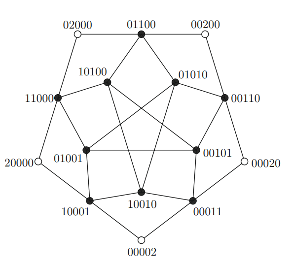
Example 4.5. Consider the graph \(G=C_5\) and its supertoken graph \({\cal F}_2(C_5)\) (the latter is represented in Figure 3). One can check that \(\dim(C_5)=2\), whereas \(\dim({\cal F}_2(C_5))=4\). The distance matrix of \(C_5\) is the following circulant matrix: \[\mbox{ $D$}=\mathop{\mathrm{circ}}(0,1,2,2,1)=\left( \begin{array}{ccccc} 0 & 1 & 2 & 2 & 1\\ 1 & 0 & 1 & 2 & 2\\ 2 & 1 & 0 & 1 & 2\\ 2 & 2 & 1 & 0 & 1\\ 1 & 2 & 2 & 1 & 0 \end{array} \right).\]
Thus, by using Theorem 1.1(ii), we see that \(\mbox{ $D$}(C_5)\) is nonsingular and, consequently, by Theorem 4.4, \(C=\{20000,02000,00200,00020,00002\}\) is a resolving set of \({\cal F}_2(C_5)\). Thus, let us check that the positions of the vertices \(\mbox{ $x$}=x_1x_2x_3x_4x_5=(x_1,x_2,x_3,x_4,x_5)\) with respect to \(C\), that is, \(\mbox{ $\rho$}(\mbox{ $x$})=\mbox{ $x$}\mbox{ $D$}\), where \(x_i\in\{0,1,2\}\) and \(\sum\limits_{i=1}^5 x_i=2\), are all different. (The five vertices \(\mbox{ $x$}\) with the same pattern, up to right shift, are the rows of the matrices on the left): \[\begin{aligned} & \left( \begin{array}{ccccc} 2& 0 & 0 & 0 & 0\\ 0 & 2 & 0 & 0 & 0\\ 0 & 0 & 2 & 0 & 0\\ 0 & 0 & 0 & 2 & 0\\ 0 & 0 & 0 & 0 & 2 \end{array} \right)\left( \begin{array}{ccccc} 0 & 1 & 2 & 2 & 1\\ 1 & 0 & 1 & 2 & 2\\ 2 & 1 & 0 & 1 & 2\\ 2 & 2 & 1 & 0 & 1\\ 1 & 2 & 2 & 1 & 0 \end{array} \right)=\left( \begin{array}{ccccc} 0 & 2 & 4 & 4 & 2\\ 2 & 0 & 2 & 4 & 4\\ 4 & 2 & 0 & 2 & 4\\ 4 & 4 & 2 & 0 & 2\\ 2 & 4 & 4 & 2 & 0 \end{array} \right), \\ & \left( \begin{array}{ccccc} 1 & 1 & 0 & 0 & 0\\ 0 & 1 & 1 & 0 & 0\\ 0 & 0 & 1 & 1 & 0\\ 0 & 0 & 0 & 1 & 1\\ 1 & 0 & 0& 0 & 1 \end{array} \right)\left( \begin{array}{ccccc} 0 & 1 & 2 & 2 & 1\\ 1 & 0 & 1 & 2 & 2\\ 2 & 1 & 0 & 1 & 2\\ 2 & 2 & 1 & 0 & 1\\ 1 & 2 & 2 & 1 & 0 \end{array} \right)=\left( \begin{array}{ccccc} 1 & 1 & 3 & 4 & 3\\ 3 & 1 & 1 & 3 & 4\\ 4 & 3 & 1 & 1 & 3\\ 3 & 4 & 3 & 1 & 1\\ 1 & 3 & 4 & 3 & 1 \end{array} \right), \\ & \left( \begin{array}{ccccc} 1 & 0 & 1 & 0 & 0\\ 0 & 1 & 0 & 1 & 0\\ 0 & 0 & 1 & 0 & 1\\ 1 & 0 & 0 & 1 & 0\\ 0 & 1 & 0 & 0 & 1 \end{array} \right)\left( \begin{array}{ccccc} 0 & 1 & 2 & 2 & 1\\ 1 & 0 & 1 & 2 & 2\\ 2 & 1 & 0 & 1 & 2\\ 2 & 2 & 1 & 0 & 1\\ 1 & 2 & 2 & 1 & 0 \end{array} \right)=\left( \begin{array}{ccccc} 2 & 2 & 2 & 3 & 3\\ 3 & 2 & 2 & 2 & 3\\ 3 & 3 & 2 & 2 & 2\\ 2 & 3 & 3 & 2 & 2\\ 2 & 2 & 3 & 3 & 2 \end{array} \right). \end{aligned}\]
As claimed, the positions of the vertices (rows of the matrices on the right) are all distinct.
Returning to the proof of Theorem 4.4, if the distance matrix \(\mbox{ $D$}\) is singular, we cannot guarantee that the set \(C\) in (5) is a resolving set. To illustrate this fact, we present the following example.
Example 4.6. Consider the graph \(G=C_6\) and its supertoken graph \({\cal F}_2(C_6)\). The cycle \(C_6\) has vertices \(1,2,\ldots,6\) with distance matrix \[\mbox{ $D$}=\mathop{\mathrm{circ}}(0,1,2,3,2,1)=\left( \begin{array}{cccccc} 0 & 1 & 2 & 3 & 2 & 1\\ 1 & 0 & 1 & 2 & 3 & 2\\ 2 & 1 & 0 & 1 & 2 & 3\\ 3 & 2 & 1 & 0 & 1 & 2\\ 2 & 3 & 2 & 1 & 0 & 1\\ 1 & 2 & 3 & 2 & 1 & 0 \end{array} \right).\]
Again, by applying Theorem 1.1(ii), we observe that \(\det\mbox{ $D$}=0\) and, hence, \(\mbox{ $D$}\) is singular. Thus, if we take the set \(C=\{200000,020000,\ldots,000002\}\), the position of the vertices \(\mbox{ $x$}_1=14=(1,0,0,1,0,0)\), \(\mbox{ $x$}_2=25=(0,1,0,0,1,0\), and \(x_3=36=(0,0,1,0,0,1)\) of \(C\) turns out to have the same \[\mbox{ $\rho$}(x_i|C)=\mbox{ $x$}_i\mbox{ $D$}=(3,3,3,3,3,3)\quad \mbox{for $i=1,2,3$,}\] showing that \(C\) is not a resolving set.
The second and third authors’ research has been supported by AGAUR from the Catalan Government under project 2021SGR00434 and MICINN from the Spanish Government under project PID2020-115442RB-I00. The research of the third author was also supported by a grant from the Universitat Politècnica de Catalunya with references AGRUPS-2024.