This study extends the concept of competition graphs to cubic fuzzy competition graphs by introducing additional variations including cubic fuzzy out-neighbourhoods, cubic fuzzy in-neighbourhoods, open neighbourhood cubic fuzzy graphs, closed neighbourhood cubic fuzzy graphs, cubic fuzzy (k) neighbourhood graphs and cubic fuzzy [k]-neighbourhood graphs. These variations provide further insights into the relationships and competition within the graph structure, each with its own defined characteristics and examples. These cubic fuzzy CMGs are further classified as cubic fuzzy k-competition graphs that show competition in the \(k\)th order between components, \(p\)-competition cubic fuzzy graphs that concentrate on competition in terms of membership degrees, and \(m\)-step cubic fuzzy competition graphs that analyze competition in terms of steps. Further, some related results about independent strong vertices and edges have been obtained for these cubic fuzzy competition graph classes. Finally, the proposed concept of cubic fuzzy competition graphs is supported by a numerical example. This example showcases how the framework of cubic fuzzy competition graphs can be practically applied to the predator-prey model to illustrate the representation and analysis of ambiguous information within the graph structures.
Graphs are mathematical structures that are used to represent pairwise relationships between items. The term ‘graph’ was first used by Euler in the 18th century while working to solve the Königsberg Bridge Problem. The first directed graph was vocally exploited by Aristotle to develop persuasive arguments. Numerous industries, including data mining, image sensing, and clustering. The main purpose of a graph is to create a relationship between distinct members of a set.
Zadeh [1] introduced the innovative concept of fuzzy sets (FSs) to deal with uncertainties a fuzzy set \(\mu\) is a mapping \(\mu : \mathcal{V} \rightarrow [0, 1].\)) The term fuzzy graphs (FGs) was announced by Rosenfeld [2] and Gehrke [3] et al. is defined as let \(G = (\mathcal{V}, \mu, \lambda)\) on universe of discourse \(\mathcal{V}\), is a FG if \(\mu\) is a fuzzy set in \(\mathcal{V}\) and \(\lambda\) is a fuzzy relation on \(\mu\) such that \(\lambda(t, u) \leq \min \{\mu(t), \mu(u)\}\) for all \(t, u \in \mathcal{V}.\) A fuzzy directed graph on a non-empty set \(\mathcal{V}\) is of the form \(\vec{{G}} = (\mathcal{V}, \mu, \lambda),\) where \(\mu\) is a fuzzy set on \(\mathcal{V}\) and \(\lambda\) is a fuzzy relation on \(\mathcal{V}\) such that \({\lambda}(\overrightarrow{t, u}) \leq \min \{\mu(t), \mu(u)\}\) for all \(t, u \in \mathcal{V}.\)
To cope with the problem of ambiguous data in different variations, Jun et al. [4] introduced the idea of cubic sets, an extended form of fuzzy sets. A CS is basically a combination of two sets, IVFSs and FSs. The term cubic graphs with its applications was introduced by Rashid et al. [5]. Cohen [6], originate the idea of competition graphs (CMGs) as the competition between species in ecology. The CMG \(C(\vec{{G}})\) of a directed graph \(\vec{{G}} = (\mathcal{V}, \mathfrak{E})\) is defined as an undirected graph \(C(\vec{{G}}) = (\mathcal{V}, \mathfrak{E})\) which has the same vertex set \(\mathcal{V}\) and contains an edge between two distinct vertices \(t, u \in \mathcal{V}\) if a vertex \(z \in \mathcal{V}\) and arcs \((\overrightarrow{t, z})\) and \((\overrightarrow{u, z}) \in \mathfrak{E}\) exist in \(\vec{{G}}\). A graph \({G}\) is said to be a CMG if a directed graph \(\vec{{G}}\) exists such that \(C(\vec{{G}}) = {G}\). Cohen’s theory was founded on the idea that if two species share the same prey, they will fight over it. Akram et al. [7] described extension of competition graphs under complex fuzzy environment and purposed the concept of bipolar fuzzy competition graphs and discussed their further properties in [8,9]. Borzooei et al. introduced new concepts of vague competition graphs in [10].
Additionally, CMGs in ecosystems have numerous uses in a variety of domains, including modelling economic centre structures, coding, energy efficiency, fuzzy logic, and fuzzy inference. The literature has developed several distinctions for these graphs, including p-CMGs of digraph [11-15], common enemy graphs of digraph [16], competition hypergraphs [17], tolerance CMGs [18] and m-step CMGs [19].
Much work has been done on CMGs whose vertices and edges are assumed to be fully specified, drawing heavily on food web models of natural communities. Whatever the case, this presumption is insufficient to represent competition in some genuine scenarios, such as a biological system where species can be weak, strong, vegetarian omnivorous, etc., and prey can be dangerous, edible, tasty, etc. It is natural to plan a fuzzy model of the CMG because species, prey, and their associations are not accurately shown.
In addition, Samanta and Pal proposed the idea of different categories of CMGs [20-22] such as fuzzy out-neighbourhood and in-neighbourhood of a vertex and of a graph are defined as follows. Let \(\vec{{G}} = (\mathcal{V}, \mu, \lambda)\) be a directed FG. Then the fuzzy out-neighbourhood of a vertex \(t\) is the fuzzy set \(\mathcal{N}^+(t)=(V^{+}_{t},s^{+}_t),\) where \(V^{+}_{t}= \{u|\lambda(\overrightarrow{t,u})>0\}\) and \(s^{+}_t: V^{+}_{t}\rightarrow[0,1]\) defined by \(s^{+}_t =\lambda(\overrightarrow{t,u})\). In similar way the fuzzy in-neighbourhood of a vertex \(t\) is the CS \(\mathcal{N}^-(t)=(V^{-}_{t}, s^{-}_t),\) where \(V^{-}_{t}= \{u|\lambda(\overrightarrow{t,u})>0\}\) and \(s^{-}_t:V^{-}_{t}\rightarrow[0,1]\) defined by \(s^{-}_t =\lambda(\overrightarrow{t,u}).\) The fuzzy neighbourhood of a vertex \(t \in \mathcal{V}\) of a directed fuzzy graph \(\vec{{G}} = (\mathcal{V}, \mu, \lambda)\) is defined as the fuzzy set \(\mathcal{N}(t) = (V_{t}, s_t),\) where \(V_{t} = \{w \mid \lambda(\overrightarrow{t, w}) > 0\}\) and \(s_t: V_{t} \rightarrow [0, 1]\) is given by \(s_t(w) = \lambda(\overrightarrow{t, w})\). The \(m\)-step fuzzy out-neighbourhood of a vertex \(t \in \mathcal{V}\) of a fuzzy directed graph \(\vec{{G}}=(\mathcal{C}, \mathcal{D})\) is defined as the fuzzy set \(\mathcal{N}^+_m(t) = (V^+_t, s^+_t),\) where \(V^+_t = \{u \mid p_m(\overrightarrow{t, u}) = \min\{\lambda(\overrightarrow{t, u_1}), \lambda(\overrightarrow{u_1, u_2}), \ldots, \lambda(\overrightarrow{u_m, u})\} > 0\}\), with \(t u_1 u_2 \ldots u_m u\) being a path from \(t\) to \(u\) and \(s^+_t: V^+_t \rightarrow [0, 1]\) is defined by \(s^+_t(u) = p_m(\overrightarrow{t, u})\). If there are multiple fuzzy paths of length \(m\), the minimum degree of membership path \({p_m}(\overrightarrow{t, u})\) should be taken.
Parvathi et al. [23] proposed intuitionistic fuzzy graphs and Sahoo and Pal [24] converted them into intuitionistic fuzzy competition graphs. Nasir et al. [25] discussed their further properties. Pal et al. [26] discuss further properties of fuzzy graphs in the book “Modern trends in fuzzy graph theory”. Pramanik discussed an extension of fuzzy competition graph and its uses in manufacturing industries in [27]. Further, Talebi et al. [28] recognized the notion of interval-valued intuitionistic fuzzy CMGs. Akram and Nasir [29] discussed interval-valued neutrosophic CMGs. Rashid et al. [5] introduced the graphical structures of CSs with real-world applications. Further, Muhiuddin et al. [] discussed cubic graphs with their properties and applications. Moreover, different extensions of cubic graphs have been discussed in [31-33]. The limitations of existing models, such as traditional fuzzy graphs and interval-valued intuitionistic fuzzy graphs, lie in their inability to effectively manage the multifaceted nature of real-world data. These models fall short in scenarios where the data exhibits both fuzziness and interval uncertainty simultaneously. Particularly, in ecological and biological systems, species interactions are often characterized by various degrees of uncertainty and vagueness, which cannot be captured by a single type of fuzzy set. Cubic fuzzy graphs provide a robust framework that combines both fuzzy membership functions and interval-valued fuzzy membership functions, allowing for a more comprehensive representation of these interactions. This dual capability enables cubic fuzzy graphs to model a wider range of real-world scenarios more effectively. This motivates us to the occurrence of cubic fuzzy CMGs. Following is a description of this study’s major goal:
Cubic FS is a useful extension of FS and IVFS which can indicate the issue with ambiguity in a single set. The cubic FS not only grasp the fuzzy information but also deals with interval-valued fuzzy data.
The proposed CMGs under cubic fuzzy environment overcome the limitations of other existing CMGs. We introduce the idea of cubic fuzzy CMGs in the current study, which deal with both fuzzy membership functions and interval-valued fuzzy membership functions. Further, we provide cubic fuzzy k-competition and cubic fuzzy p-CMGs, two extensions of cubic fuzzy CMGs. Also, we define m-step cubic fuzzy CMGs, m-step fuzzy neighbourhood graphs, and cubic fuzzy neighbourhood graphs. Finally, to emphasise the cubic fuzzy CMG’s importance in the actual world, we present an application.
This paper is classified as follows: Section 2, includes a few elementary definitions which have a key role in the development of cubic fuzzy CMGs. Furthermore, the innovative concept of cubic fuzzy CMGs with its two valuable expansions namely, cubic fuzzy k-CMGs and p-competition cubic FGs was demonstrated. Section 3 contains the notion of cubic fuzzy neighbourhood graphs in addition to some related results. Section 4, m-step cubic fuzzy CMGs defined and related results are obtained. Section 5 includes the usefulness of cubic fuzzy CMGs to highlight the significance of these graphs in a practical manner.
In this section, preliminary definitions and properties of cubic CMGs and its different variations like cubic Fuzzy k-CMGs and p-Competition Cubic FGs have been explored.
Definition 1. [4] Let \(\mathcal{V}\) be a universe set. A CS \(\mathcal{C}\) is a structure; \[\label{1} \mathcal{C} = \{(t, \mu(t), \lambda(t)) ~|~t \in \mathcal{V}\},\tag{1}\] where \(\mu(t)=[\mu^L(t), \mu^U(t)],\) represents the interval valued fuzzy membership over \(\mathcal{V},\) while \(\lambda(t)\) represents simple fuzzy degree of membership.
Definition 2. The support of CS \(\mathcal{C} = \{(t, \mu(t), \lambda(t)) ~|~t \in \mathcal{V}\},\) in \(\mathcal{V}\) is basically a subset \(\mathcal{C}_o\) of \(\mathcal{V}\) defined by \(\mathcal{C}_o= \{t \in \mathcal{V} : \mu_{\mathcal{C}}(t)\neq0~ and ~ \lambda_{\mathcal{C}}(t)\neq 0\}\) and \(|supp(\mathcal{C}_0)|\) is the total number of elements present in the set.
Definition 3. The height of CS \(\mathcal{C}\) in \(\mathcal{V}\) is defined as:\[\begin{aligned} % \nonumber to remove numbering (before each equation) h(\mathcal{C}) &=& ([\sup\limits_{t\in \mathcal{V}}\mu^{L}_\mathcal{C}(t,u), \sup\limits_{t\in \mathcal{V}}\mu^{U}_\mathcal{C}(t,u)], \sup\limits_{t\in \mathcal{V}}\lambda_\mathcal{C}(t,u)), \end{aligned}\] for all \(t\in \mathcal{V}.\)
The concept of cubic sets can be extended to the concept of a cubic fuzzy graph, which combines cubic sets with graph theory. A cubic fuzzy graph extends the fuzzy graph concept by incorporating interval-valued memberships, providing a richer framework for modeling uncertainty and vagueness in graph structures.
Definition 4. [5] A cubic fuzzy graph \({G}=(\mathcal{C}, \mathcal{D})\) of a graph \({G}=(\mathcal{V}, \mathfrak{E}),\) where \(\mathcal{C}=(\mu_\mathcal{C}, \lambda_\mathcal{C})\) represents the vertex set and \(\mathcal{D}=(\mu_\mathcal{D}, \lambda_\mathcal{D})\) represents an edge set, holds the following conditions:
The functions \(\mu_\mathcal{C} : \mathcal{V} \rightarrow [0, 1]\times [0, 1]\) and \(\lambda_\mathcal{C} : \mathcal{V} \rightarrow [0, 1]\) represent the interval-valued membership degrees and simple fuzzy valued membership degrees, respectively.
The functions \(\mu_\mathcal{D} : \mathcal{V} \times \mathcal{V} \rightarrow [0, 1]\times [0, 1]\) and \(\lambda_\mathcal{D} : \mathcal{V} \times \mathcal{V}\rightarrow [0, 1]\) are denoted by: \[\mu^L_\mathcal{D}(t,u)\leq \mu^L_\mathcal{C}(t)\wedge \mu^L_\mathcal{C}(u),\] \[\mu^U_\mathcal{D}(t,u)\leq \mu^U_\mathcal{C}(t)\wedge \mu^U_\mathcal{C}(u),\] \[\lambda_\mathcal{D}(t,u)\leq \lambda_\mathcal{C}(t)\wedge \lambda_\mathcal{C}(u).\]
\(\rm for~all ~(t,u) \in \mathcal{E}\subseteq \mathcal{V} \times \mathcal{V},\) where \(\mu^L_\mathcal{D}\) and \(\mu^U_\mathcal{D}\) are the lower and upper values of the interval valued membership, respectively.
Definition 5. The edge of a cubic graph denoted as \((t,u)\) is called independent strong if: \[\begin{aligned} % \nonumber to remove numbering (before each equation) \mu^L_\mathcal{D}(t,u) &\geq & \frac{\mu^L_\mathcal{C}(t)\wedge\mu^L_\mathcal{C}(u)}{2},\\ \mu^U_\mathcal{D}{(t,u)} &\geq& \frac{\mu^U_\mathcal{C}(t)\wedge\mu^U_\mathcal{C}(u)}{2},\\ \lambda_{\mathcal{D}}{(t,u)} &\geq&\frac{\lambda_\mathcal{C}(t)\wedge\lambda_\mathcal{C}(u)}{2}. \end{aligned}\]
Definition 6. The cubic graph is said to be complete if: \[\begin{aligned} % \nonumber to remove numbering (before each equation) \mu^L_\mathcal{D}(t,u) &= & \frac{\mu^L_\mathcal{C}(t)\wedge\mu^L_\mathcal{C}(u)}{2},\\ \mu^U_\mathcal{D}{(t,u)} &=& \frac{\mu^U_\mathcal{C}(t)\wedge\mu^U_\mathcal{C}(u)}{2}, \\ \lambda_{\mathcal{D}}{(t,u)} &=&\frac{\lambda_\mathcal{C}(t)\wedge\lambda_\mathcal{C}(u)}{2}. \end{aligned}\]
Further, we define a cubic directed graph (CuDG), a directed version of the cubic fuzzy graph.
Definition 7. A cubic directed graph (CuDG) on a set \(\mathcal{V}\) is defined as \(\vec{{G}} = (\mathcal{C}, \mathcal{D}),\) where \(\mathcal{C} = (\mu_\mathcal{C}, \lambda_\mathcal{C})\) represents the vertex set and \(\mathcal{D} = (\mu_\mathcal{D}, \lambda_\mathcal{D})\) represents the edge set, such that: \[\begin{aligned} \mu^L_\mathcal{D}(\overrightarrow{t, u}) &\leq \mu^L_\mathcal{C}(t) \wedge \mu^L_\mathcal{C}(u), \\ \mu^U_\mathcal{D}(\overrightarrow{t, u}) &\leq \mu^U_\mathcal{C}(t) \wedge \mu^U_\mathcal{C}(u), \\ \lambda_\mathcal{D}(\overrightarrow{t, u}) &\leq \lambda_\mathcal{C}(t) \wedge \lambda_\mathcal{C}(u). \end{aligned}\]
To understand the interaction between vertices in a CuDG, the notions of cubic fuzzy out-neighborhood and in-neighborhood describing the set of vertices that are directly connected to a given vertex through directed edges is defined as follows.
Definition 8. Consider a CuDG \(\vec{{G}} = (\mathcal{C}, \mathcal{D})\). The cubic fuzzy out-neighbourhood for any vertex \(t\) is defined as the CS \(\mathcal{N}^+(t) = (V^+_t, r^+_t, s^+_t),\) where \(V^+_t = \{u \mid \mu^L_{\mathcal{D}}(\overrightarrow{t, u}) > 0, \lambda_{\mathcal{D}}(\overrightarrow{t, u}) > 0\}\) and \(r^+_t : V^+_t \rightarrow [0, 1] \times [0, 1]\) is given by \(r^+_t(u) = [\mu^L_{\mathcal{D}}(\overrightarrow{t, u}), \mu^U_{\mathcal{D}}(\overrightarrow{t, u})]\) and \(s^+_t : V^+_t \rightarrow [0, 1]\) is given by \(s^+_t(u) = \lambda_{\mathcal{D}}(\overrightarrow{t, u})\).
Similarly, the cubic fuzzy in-neighbourhood for any vertex \(t\) is defined as the CS \(\mathcal{N}^-(t) = (V^-_t, r^-_t, s^-_t),\) where \(V^-_t = \{u \mid \mu^L_{\mathcal{D}}(\overrightarrow{u, t}) > 0, \lambda_{\mathcal{D}}(\overrightarrow{u, t}) > 0\}\) and \(r^-_t : V^-_t \rightarrow [0, 1] \times [0, 1]\) is given by \(r^-_t(u) = [\mu^L_{\mathcal{D}}(\overrightarrow{u, t}), \mu^U_{\mathcal{D}}(\overrightarrow{u, t})]\) and \(s^-_t : V^-_t \rightarrow [0, 1]\) is given by \(s^-_t(u) = \lambda_{\mathcal{D}}(\overrightarrow{u, t})\).
The theoretical basis of cubic CMGs like cubic fuzzy in-neighbourhood and cubic fuzzy out-neighbourhood for any vertex sets are obtained. Next, we will see practical example to illustrate these definitions.
Example 1. Let \(\vec{{G}}=(\mathcal{C}, \mathcal{D})\) be a CuDG on the vertex set \(\mathcal{V}=\{p,q,r,s,t\}\) as shown in Figure 1.
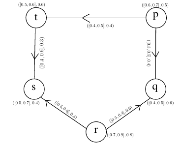
The degree of memberships of the vertices as well as edges are chosen arbitrarily as described in Figure 1. The cubic fuzzy out neighbourhood and cubic fuzzy in neighbourhood are shown in Table 1:
| \(t\) | \(\mathcal{N}^+(t)\) | \(\mathcal{N}^-(t)\) |
| p | {(t,[0.4,0.5],0.4),(q,[0.3,0.5],0.4)} | Ø |
| q | Ø | {(p,[0.3,0.5],0.4),(q,[0.3,0.4],0.6)} |
| r | {(s,[0.5,0.6],0.4),(q,[0.3,0.4],0.6)} | Ø |
| s | Ø | {(t,[0.4,0.6],0.3),(r,[0.5,0.6],0.4)} |
| t | {(s,[0.4,0.6],0.3)} | {(p,[0.4,0.5],0.4)} |
Now, we are going to define the definition of cubic fuzzy CMG.
Definition 9. The cubic fuzzy CMG \(C(\vec{{G}})\) of CuDG \(\vec{{G}}=({\mathcal{C}}, \mathcal{D})\) is an undirected graph \({G}= ({\mathcal{C}}, {\mathcal{D}})\) with \({\mathcal{C}}({G})=\mathcal{C}(\vec{{G}})\) and \({\mathcal{D}}({G})=\{(t,u);\mathcal{N}^+(t)\cap\mathcal{N}^+(u) >0\}.\) The degree of memberships of the edge \((t,u)\) in \(C(\vec{{G}})\) are: \[\begin{aligned} % \nonumber to remove numbering (before each equation) \mu^L_\mathcal{D}(t,u) &=& (\mu^L_{\mathcal{C}}(t)\wedge\mu^L_{\mathcal{C}}(u))h^L(\mathcal{N}^+(t)\cap\mathcal{N}^+(u)),\\ \mu^U_\mathcal{D}{(t,u)} &=& (\mu^U_{\mathcal{C}}(t)\wedge\mu^U_{\mathcal{C}}(u))h^U(\mathcal{N}^+(t)\cap\mathcal{N}^+(u)),\\ \lambda_{\mathcal{D}}{(t,u)} &=&(\lambda_{\mathcal{C}}(t)\wedge\lambda_{\mathcal{C}}(u))h(\mathcal{N}^+(t)\cap\mathcal{N}^+(u)). \end{aligned}\]
Example 2. Consider a CuDG \(\vec{{G}}=(\mathcal{C}, \mathcal{D})\) on vertex set \(\mathcal{V}=\{a,b,c,d,e,f\}\) as shown in Figure 2.
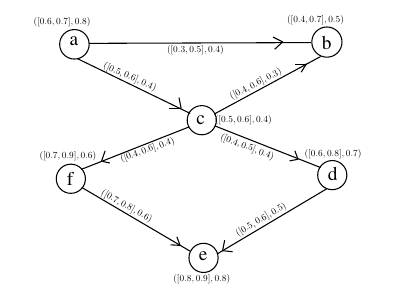
The degree of memberships of the vertices and edges are taken arbitrarily as described in Figure 2. The cubic fuzzy out neighbourhood vertices are: \(\mathcal{N}^+(a)=\{(b,[0.3,0.5],0.4),(c,[0.5,0.7],0.4)\},\) \(\mathcal{N}^+(b)={\O},\) \(\mathcal{N}^+(c)=\{(b,[0.4,0.6],0.3),(d,[0.4,0.5],0.4),(f,[0.4,0.6],0.4)\},\) \(\mathcal{N}^+(d)=\{(e,[0.5,0.6],0.5\},\) \(\mathcal{N}^+(e)={\O},\) \(\mathcal{N}^+(f)=\{(e,[0.7,0.8],0.6)\}.\)
Since, \[\mathcal{N}^+(a)\cap\mathcal{N}^+(c)=\{(b,[0.3,0.5],0.3)\},\] and \[\mathcal{N}^+(d)\cap\mathcal{N}^+(f)=\{(e,[0.5,0.6],0.5)\}.\] Therefore, \(h^L(\mathcal{N}^+(a)\cap\mathcal{N}^+(c))=0.3,\) \(h^U(\mathcal{N}^+(a)\cap\mathcal{N}^+(c))=0.5,\) \(h(\mathcal{N}^+(a)\cap\mathcal{N}^+(c))=0.3\) and \(h^L(\mathcal{N}^+(d)\cap\mathcal{N}^+(f))=0.5,\) \(h^U(\mathcal{N}^+(d)\cap\mathcal{N}^+(f))=0.6,\) \(h(\mathcal{N}^+(d)\cap\mathcal{N}^+(f))=0.5.\)
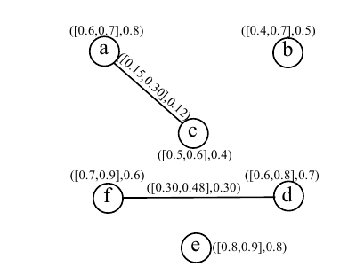
Thus, there exist edges among vertices \(a, c\) and \(d, f\) in cubic fuzzy CMG \(C(\vec{{G}})\), whose degree of memberships are given by: \(\mu^L_\mathcal{D}(a, c)=0.15,\) \(\mu^U_\mathcal{D}(a, c)=0.30,\) \(\lambda_\mathcal{D}(a, c)=0.12\) and \(\mu^L_\mathcal{D}(d, f)=0.30,\) \(\mu^U_\mathcal{D}(d, f)=0.48,\) \(\lambda_\mathcal{D}(d, f)=0.30.\) For all remaining edges \(\mu^L_\mathcal{D}=\mu^U_\mathcal{D}=\lambda_\mathcal{D}=0.\) The corresponding cubic fuzzy CMG is shown in Figure 3.
Theorem 1. Let \(\vec{{G}}=(\mathcal{C}, \mathcal{D})\) be a CuDG and \({G}= ({\mathcal{C}}, {\mathcal{D}})\) be its CMG. An edge \((t,u)\) in \(C(\vec{{G}})\) is independent strong if and only if \(h^L(\mathcal{N}^+(t)\cap\mathcal{N}^+(u))> 0.5,\) \(h^U(\mathcal{N}^+(t)\cap\mathcal{N}^+(u))> 0.5\) and \(h(\mathcal{N}^+(t)\cap\mathcal{N}^+(u))> 0.5\) provided that \(\mathcal{N}^+(t)\cap\mathcal{N}^+(u)\) has one and only one element.
Proof. Since, \(\mathcal{N}^+(t)\cap\mathcal{N}^+(u)\) has one and only one element. Let \(\mathcal{N}^+(t)\cap\mathcal{N}^+(u)= \{( m, [a, \breve{a}] , c)\},\) where \([a,\breve{a}]\) are interval-valued fuzzy membership of the vertex \(m.\) Then \(h^L(\mathcal{N}^+(t)\cap\mathcal{N}^+(u))= a,\) \(h^U(\mathcal{N}^+(t)\cap\mathcal{N}^+(u))= \breve{a}\) and \(h(\mathcal{N}^+(t)\cap\mathcal{N}^+(u))= c.\) So, \[\begin{aligned} % \nonumber to remove numbering (before each equation) \mu^L_\mathcal{D}(t,u) = (\mu^L_{\mathcal{C}}(t)\wedge\mu^L_{\mathcal{C}}(u))h^L(\mathcal{N}^+(t)\cap\mathcal{N}^+(u))&=& a \times (\mu^L_{\mathcal{C}}(t)\wedge\mu^L_{\mathcal{C}}(u))>\frac{1}{2} (\mu^L_{\mathcal{C}}(t)\wedge\mu^L_{\mathcal{C}}(u),\\ \mu^U_\mathcal{D}(t,u) = (\mu^U_{\mathcal{C}}(t)\wedge\mu^U_{\mathcal{C}}(u))h^U(\mathcal{N}^+(t)\cap\mathcal{N}^+(u))&=& \breve{a} \times (\mu^U_{\mathcal{C}}(t)\wedge\mu^U_{\mathcal{C}}(u))>\frac{1}{2} (\mu^U_{\mathcal{C}}(t)\wedge\mu^U_{\mathcal{C}}(u),\\ \lambda_{\mathcal{D}}{(t,u)}=(\lambda_{\mathcal{C}}(t)\wedge\lambda_{\mathcal{C}}(u))h(\mathcal{N}^+(t)\cap\mathcal{N}^+(u)) &=& c \times (\lambda_{\mathcal{C}}(t)\wedge\lambda_{\mathcal{C}}(u))>\frac{1}{2}(\lambda_{\mathcal{C}}(t)\wedge\lambda_{\mathcal{C}}(u)). \end{aligned}\] Hence, the edge \((t,u)\) in \(C(\vec{{G}})\) is independent strong if and only if \(a>0.5,\) \(\breve{a}>0.5\) and \(c>0.5.\) ◻
Theorem 2. If all the edges of a CuDG \(\vec{{G}}=({\mathcal{C}}, \mathcal{D})\) be independent strong, then \(\frac{\mu^L_\mathcal{D}(t,u)}{(\mu^L_{\mathcal{C}}(t)\wedge\mu^L_{\mathcal{C}}(u))^2}>0.5,\) \(\frac{\mu^U_\mathcal{D}(t,u)}{(\mu^U_{\mathcal{C}}(t)\wedge\mu^U_{\mathcal{C}}(u))^2}>0.5\) and \(\frac{\lambda_\mathcal{D}(t,u)}{(\lambda_{\mathcal{C}}(t)\wedge\lambda_{\mathcal{C}}(u))^2}>0.5\) for all \(t,u \in \mathcal{V}\) in \(C(\vec{{G}}),\) provided \((\mu^L_{\mathcal{C}}(t)\wedge\mu^L_{\mathcal{C}}(u))\neq0,\) \((\mu^U_{\mathcal{C}}(t)\wedge\mu^U_{\mathcal{C}}(u))\neq0\) and \(\lambda_{\mathcal{C}}(t)\wedge\lambda_{\mathcal{C}}(u))\neq0.\)
Proof. Since, all the edges of \(\vec{{G}}=({\mathcal{C}}, \mathcal{D})\) be independent strong, then \(\mu^L_\mathcal{D}(\overrightarrow{t,u})\geq\frac{\mu^L_{\mathcal{C}}(t)\wedge\mu^L_{\mathcal{C}}(u)}{2},\) \(\mu^U_\mathcal{D}(\overrightarrow{t,u})\geq\frac{\mu^U_{\mathcal{C}}(t)\wedge\mu^U_{\mathcal{C}}(u)}{2}\) and \(\lambda_\mathcal{D}(\overrightarrow{t,u})\geq\frac{\lambda_{\mathcal{C}}(t)\wedge\lambda_{\mathcal{C}}(u)}{2},\) i.e \(\frac{\mu^L_\mathcal{D}(\overrightarrow{t,u})}{\mu^L_{\mathcal{C}}(t)\wedge\mu^L_{\mathcal{C}}(u)}\geq0.5,\) \(\frac{\mu^U_\mathcal{D}(\overrightarrow{t,u})}{\mu^U_{\mathcal{C}}(t)\wedge\mu^U_{\mathcal{C}}(u)}\geq0.5\) and \(\frac{\lambda_\mathcal{D}(\overrightarrow{t,u})}{\lambda_{\mathcal{C}}(t)\wedge\lambda_{\mathcal{C}}(u)}\geq0.5,\) for all \(t,u \in V\) such that \(\mu^L_\mathcal{D}(t,u)\neq0,\) \(\mu^U_\mathcal{D}(t,u)\neq0\) and \(\lambda_\mathcal{D}(t,u)\neq0.\) Let \(\mathcal{N}^+(t)\cap\mathcal{N}^+(u)\) has at least one element. Let \[\label{8} \mathcal{N}^+(t)\cap\mathcal{N}^+(u)= \{( m_i, [a_i, \breve{a_i}] , c_i)|i= 1,\ldots k\},\tag{2}\] where \([a_i, \breve{a_i}]\) is interval-valued membership and \(c_i\) is simple fuzzy degree of membership of \(m_i, (i=1,\ldots k).\) This shows that \[[a_i, \breve{a_i}]=[\min\{\mu^L_\mathcal{D}(\overrightarrow{t,m_i}),\mu^L_\mathcal{D}(\overrightarrow{u,m_i})\}, \min \{\mu^U_{\mathcal{D}}(\overrightarrow{t,m_i}),\mu^U_{\mathcal{D}}(\overrightarrow{u,m_i})\}]\] \[c_i=\min\{\lambda_{\mathcal{D}}(\overrightarrow{t,m_i}),\lambda_{\mathcal{D}}(\overrightarrow{u,m_i})\}.\] Therefore, \[h^L(\mathcal{N}^+(t)\cap\mathcal{N}^+(u))= \max\{a_1, a_2,\ldots,a_k\}=a_{\max},\] \[h^U(\mathcal{N}^+(t)\cap\mathcal{N}^+(u))= \max\{\breve{a_1}, \breve{a_2},\ldots,\breve{a_k}\}=\breve{a}_{\max},\] \[h(\mathcal{N}^+(t)\cap\mathcal{N}^+(u))= \max\{c_1, c_2,\ldots,c_k\}=c_{\max}.\] Obviously, \(a_{\max}>\mu^L_{\mathcal{D}}(\overrightarrow{t,u})\) \(\breve{a}_{\max}>\mu^U_{\mathcal{D}}(\overrightarrow{t,u})\) and \(c_{\max}>\lambda_{\mathcal{D}}(\overrightarrow{t,u}),\) shows that: \[\frac{a_{\max}}{\mu^L_{\mathcal{C}}(t)\wedge\mu^L_{\mathcal{C}}(u)}>\frac{\mu^L_{\mathcal{D}}(\overrightarrow{t,u})} {\mu^L_{\mathcal{C}}(t)\wedge\mu^L_{\mathcal{C}}(u)}\geq 0.5\] \[\frac{\breve{a}_{\max}}{\mu^U_{\mathcal{C}}(t)\wedge\mu^U_{\mathcal{C}}(u)}>\frac{\mu^U_{\mathcal{D}}(\overrightarrow{t,u})} {\mu^U_{\mathcal{C}}(t)\wedge\mu^U_{\mathcal{C}}(u)}\geq 0.5\] \[\frac{c_{\max}}{\lambda_{\mathcal{C}}(t)\wedge\lambda_{\mathcal{C}}(u)}>\frac{\lambda_{\mathcal{D}}(\overrightarrow{t,u})} {\lambda_{\mathcal{C}}(t)\wedge\lambda_{\mathcal{C}}(u)}\geq 0.5.\] As, \[\mu^L_\mathcal{D}(t,u)=(\mu^L_{\mathcal{C}}(t)\wedge\mu^L_{\mathcal{C}}(u))h^L(\mathcal{N}^+(t)\cap\mathcal{N}^+(u))~or~ \frac{\mu^L_\mathcal{D}(t,u)}{\mu^L_{\mathcal{C}}(t)\wedge\mu^L_{\mathcal{C}}(u)}=a_{\max}\] \[\mu^U_\mathcal{D}{(t,u)}=(\mu^U_{\mathcal{C}}(t)\wedge\mu^U_{\mathcal{C}}(u))h^U(\mathcal{N}^+(t)\cap\mathcal{N}^+(u))~or~ \frac{\mu^U_\mathcal{D}(t,u)}{\mu^U_{\mathcal{C}}(t)\wedge\mu^U_{\mathcal{C}}(u)}=\breve{a}_{\max}\] \[\lambda_{\mathcal{D}}{(t,u)}=(\lambda_{\mathcal{C}}(t)\wedge\lambda_{\mathcal{C}}(u))h(\mathcal{N}^+(t)\cap\mathcal{N}^+(u) ~or~\frac{\lambda_\mathcal{D}(t,u)}{\lambda_{\mathcal{C}}(t)\wedge\lambda_{\mathcal{C}}(u)}=c_{\max}.\] Then, \[\frac{(\mu^L_{\mathcal{D}}(\overrightarrow{t,u}))}{(\mu^L_{\mathcal{C}}(t)\wedge\mu^L_{\mathcal{C}}(u))^2}= \frac{a_{\max}}{\mu^L_{\mathcal{C}}(t)\wedge\mu^L_{\mathcal{C}}(u)}\geq 0.5\] \[\frac{(\mu^U_{\mathcal{D}}(\overrightarrow{t,u}))} {(\mu^U_{\mathcal{C}}(t)\wedge\mu^U_{\mathcal{C}}(u))^2}=\frac{\breve{a}_{\max}}{\mu^U_{\mathcal{C}}(t)\wedge\mu^U_{\mathcal{C}}(u)}\geq 0.5\] \[\frac{(\lambda_{\mathcal{D}}(\overrightarrow{t,u}))} {(\lambda_{\mathcal{C}}(t)\wedge\lambda_{\mathcal{C}}(u))^2}=\frac{c_{\max}}{\lambda_{\mathcal{C}}(t)\wedge\lambda_{\mathcal{C}}(u)}\geq 0.5.\] ◻
It is noted that, an independent strong edge may or may not exist in the corresponding cubic fuzzy CMGs if all of a CuDG’s edges are independent strong.
In this section, the concept of fuzzy k-CMGs derived from CuDGs has been explored. Fuzzy k-CMGs extend the idea of common membership by introducing a fuzzy degree to the edges, reflecting the strength of connection based on shared neighborhoods. This approach allows for a more nuanced understanding of the relationships between vertices, especially in scenarios where connections are not merely binary but have degrees of intensity.
Definition 10. Take \(\vec{{G}}=(\mathcal{C}, \mathcal{D})\) be a CuDG and \(k\) be a non-negative number. The fuzzy k-CMG \(C_k(\vec{{G}})\) for the CuDG is an undirected graph \({G}= (\mathcal{C}, {\mathcal{D}})\) with \(\mathcal{C}(C_k({G}))=\mathcal{C}(\vec{{G}})\) and \(\mathcal{D}(C_k(\vec{{G}}))=\{(t,u);\mathcal{N}^+(t)\cap\mathcal{N}^+(u) >k\}.\) The membership degree of the edge \((t,u) \in \mathcal{V} \times \mathcal{V}\) in \(C_k(\vec{{G}})\) is calculated by: \[\begin{aligned} % \nonumber to remove numbering (before each equation) \mu^L_\mathcal{D}(t,u) &=& \frac{\check{k}-k}{k}(\mu^L_\mathcal{C}(t)\wedge\mu^L_\mathcal{C}(u))h^L(\mathcal{N}^+(t)\cap\mathcal{N}^+(u)),\\ \mu^U_\mathcal{D}{(t,u)} &=& \frac{\check{k}-k}{k}(\mu^U_\mathcal{C}(t)\wedge\mu^U_\mathcal{C}(u))h^U(\mathcal{N}^+(t)\cap\mathcal{N}^+(u)),\\ \lambda_{\mathcal{D}}{(t,u)} &=& \frac{\check{k}-k}{k}(\lambda_\mathcal{C}(t)\wedge\lambda_\mathcal{C}(u))h(\mathcal{N}^+(t)\cap\mathcal{N}^+(u)), \end{aligned}\] where \(|\mathcal{N}^+(t)\cap\mathcal{N}^+(u)|=\check{k}.\)
To better understand this concept, let‘s consider an example of CuDG and how the fuzzy k-CMG is constructed from it.
Example 3. Let \(\vec{{G}}=(\mathcal{C}, \mathcal{D})\) be a CuDG on vertex set \(\mathcal{V}=\{a,b,c,d,e,f\}\) as shown in Figure 4.
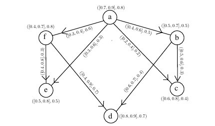
The degree of memberships of the vertices and edges are taken arbitrarily as described in Figure 4. The cubic fuzzy out neighbourhood vertices are: \(\mathcal{N}^+(a)=\{(b,[0.4,0.6],0.5),(f,[0.3,0.4],0.6),(c,[0.2,0.4],0.2),(e,[0.3,0.6],0.3)\},\) \(\mathcal{N}^+(b)=\{(c,[0.5,0.6],0.3),(d,[0.6,0.7],0.4)\},\) \(\mathcal{N}^+(c)={\O},\) \(\mathcal{N}^+(d)={\O},\) \(\mathcal{N}^+(e)={\O},\) \(\mathcal{N}^+(f)=\{(d,[0.4,0.9],0.7),(e,[0.4,0.8],0.3)\}.\) Since, \[\mathcal{N}^+(a)\cap\mathcal{N}^+(b)=\{(c,[0.2,0.4],0.2)\},\] \[\mathcal{N}^+(b)\cap\mathcal{N}^+(f)=\{(d,[0.4,0.7],0.4)\},\] \[\mathcal{N}^+(a)\cap\mathcal{N}^+(f)=\{(e,[0.3,0.6],0.3)\}.\] Therefore, \(h^L(\mathcal{N}^+(a)\cap\mathcal{N}^+(b))=0.2,\) \(h^U(\mathcal{N}^+(a)\cap\mathcal{N}^+(b))=0.4,\) \(h(\mathcal{N}^+(b)\cap\mathcal{N}^+(f))=0.2,\) \(h^L(\mathcal{N}^+(b)\cap\mathcal{N}^+(f))=0.4,\) \(h^U(\mathcal{N}^+(b)\cap\mathcal{N}^+(f))=0.7,\) \(h(\mathcal{N}^+(a)\cap\mathcal{N}^+(b))=0.4,\) \(h^L(\mathcal{N}^+(a)\cap\mathcal{N}^+(f))=0.3,\) \(h^U(\mathcal{N}^+(a)\cap\mathcal{N}^+(f))=0.6,\) \(h(\mathcal{N}^+(a)\cap\mathcal{N}^+(f))=0.3.\)
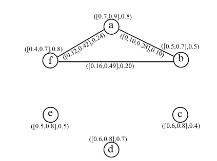
Thus, there exist edges \((a, b)\) \((b, f)\) and \((a, f)\) in cubic fuzzy \(0.2\)-CMG \(C_k(\vec{{G}})\), whose degree of memberships are given by: \(\mu^L_\mathcal{D}(a, b)=0.10,\) \(\mu^U_\mathcal{D}(a, b)=0.28,\) \(\lambda_\mathcal{D}(a, b)=0.10\) \(\mu^L_\mathcal{D}(b, f)=0.16,\) \(\mu^U_\mathcal{D}(b, f)=0.49,\) \(\lambda_\mathcal{D}(b, f)=0.20,\) \(\mu^L_\mathcal{D}(a, f)=0.12,\) \(\mu^U_\mathcal{D}(a, f)=0.42,\) \(\lambda_\mathcal{D}(a, f)=0.24.\) For all remaining edges \(\mu^L_\mathcal{D}=\mu^U_\mathcal{D}=\lambda_\mathcal{D}=0\) The corresponding cubic fuzzy \(0.2\)-CMG is shown in Figure 5.
We now proceed to a theorem that provides conditions under which an edge in the fuzzy k-CMG is considered independent and strong.
Theorem 3. Suppose \(\vec{{G}}=(\mathcal{C}, \mathcal{D})\) be a CuDG. If \(|\mathcal{N}^+(t)\cap\mathcal{N}^+(u)|>2k\) and \(h^L(\mathcal{N}^+(t)\cap\mathcal{N}^+(u))=1,\) \(h^U(\mathcal{N}^+(t)\cap\mathcal{N}^+(u))=1,\) \(h(\mathcal{N}^+(t)\cap\mathcal{N}^+(u))=1,\) then this implies that the edge \((t,u)\) is independent strong in \(C_k(\vec{{G}}).\)
Proof. Consider a CuDG \(\vec{{G}}=(\mathcal{C}, \mathcal{D})\) and \(C_k(\vec{{G}})= (\mathcal{V}, {\mathcal{C}}, {\mathcal{D}})\) be the corresponding cubic fuzzy k-CMG. Also, if \(h^L(\mathcal{N}^+(t)\cap\mathcal{N}^+(u))=1\) and \(|\mathcal{N}^+(t)\cap\mathcal{N}^+(u)|>2k,\) then, \(\check{k}>2k\) and so, \(\frac{\check{k}-k}{k}>\frac{1}{2},\) where \(\check{k}=|\mathcal{N}^+(t)\cap\mathcal{N}^+(u)|.\) Hence, \[\mu^L_\mathcal{D}(t,u)=\frac{\check{k}-k}{k}(\mu^L_{\mathcal{C}}(t)\wedge\mu^L_{\mathcal{C}}(u)) h^L(\mathcal{N}^+(t)\cap\mathcal{N}^+(u))>\frac{1}{2}(\mu^L_{\mathcal{C}}(t)\wedge\mu^L_{\mathcal{C}}(u)),\] we can write it as \[\frac{\mu^L_\mathcal{D}(t,u)}{\mu^L_{\mathcal{C}}(t)\wedge\mu^L_{\mathcal{C}}(u)}>\frac{1}{2}.\] In similar steps, it can be proved that: \(\mu^U_\mathcal{D}(t,u)>\frac{1}{2}(\mu^L_{\mathcal{C}}(t)\wedge\mu^U_{\mathcal{C}}(u)),\) and \(\lambda_\mathcal{D}(t,u)>\frac{1}{2}(\lambda_{\mathcal{C}}(t)\wedge\lambda_{\mathcal{C}}(u)).\) Hence, the edge \((t,u)\) is independent strong in \(C_k(\vec{{G}}).\) ◻
In this section, the concept of p-competition cubic FGs, which extend the classical notion of CuDGs has been introduced. This extension allows to model uncertainty and partial information in the relationships between vertices. We start by defining a p-competition cubic FG \(C^p(\vec{{G}})\) associated with a CuDG \(\vec{{G}}\):
Definition 11. Consider a positive integer \(p,\) a p-competition cubic FG \(C^p(\vec{{G}})\) of a CuDG \(\vec{{G}}=(\mathcal{C}, \mathcal{D})\) is an undirected graph \(C^p(\vec{{G}})= ({\mathcal{C}}, {\mathcal{D}})\) with \(\mathcal{C}(C^p(\vec{{G}}))=\mathcal{V}({G})\) and \(\mathcal{D}(C^p(\vec{{G}}))=\{(t,u);\mathcal{N}(t)\cap\mathcal{N}(u)\geq p\}.\) The degree of membership of \((t,u) \in \mathcal{V}\) in \(C^p(\vec{{G}})\) is calculated as: \[\begin{aligned} % \nonumber to remove numbering (before each equation) \mu^L_\mathcal{D}(t,u) &=& \frac{(n-p)+1}{n}[\mu^L_\mathcal{C}(t)\wedge\mu^L_\mathcal{C}(u)]h^L(\mathcal{N}^+(t)\cap\mathcal{N}^+(u))\\ \mu^U_\mathcal{D}{(t,u)} &=& \frac{(n-p)+1}{n}[\mu^U_\mathcal{C}(t)\wedge\mu^U_\mathcal{C}(u)]h^U(\mathcal{N}^+(t)\cap\mathcal{N}^+(u))\\ \lambda_{\mathcal{D}}{(t,u)} &=& \frac{(n-p)+1}{n}[\lambda_\mathcal{C}(t)\wedge\lambda_\mathcal{C}(u)]h(\mathcal{N}^+(t)\cap\mathcal{N}^+(u)) \end{aligned}\] where \(|supp(\mathcal{N}^+(t)\cap\mathcal{N}^+(u))|=n.\)
Example 4. Consider a CuDG \(\vec{{G}}=(\mathcal{C}, \mathcal{D})\) on vertex set \(\mathcal{V}=\{p,q,r,a,b,c\}\) as shown in Figure 6.
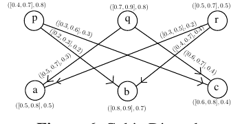
The degree of memberships of the vertices and edges are taken
arbitrarily as described in Figure 6. The cubic fuzzy out
neighbourhood vertices are:
\[\mathcal{N}^+(p)=\{(b,[0.2,0.3],0.2),(c,[0.3,0.6],0.3)\},\]
\[\mathcal{N}^+(q)=\{(a,[0.5,0.7],0.3),(c,[0.6,0.7],0.4)\},\]
\[\mathcal{N}^+(r)=\{(a,[0.3,0.5],0.2),(b,[0.4,0.7],0.4)\}.\]
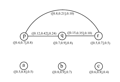
Since, \[\mathcal{N}(p)\cap\mathcal{N}(q)=\{(c,[0.3,0.6],0.3)\},\]
\[\mathcal{N}(p)\cap\mathcal{N}(r)=\{(d,[0.2,0.3],0.2)\},\]
\[\mathcal{N}(q)\cap\mathcal{N}(r)=\{(a,[0.3,0.5],0.2\}.\]
Therefore, for \(p=3,\) the
corresponding \(3\)-competition cubic
FG is shown in Figure 7.
Theorem 4. Consider a CuDG \(\vec{{G}}=(\mathcal{C}, \mathcal{D}).\) If \(h^L(\mathcal{N}^+(t)\cap\mathcal{N}^+(u))=1,\) \(h^U(\mathcal{N}^+(t)\cap\mathcal{N}^+(u))=1,\) \(h(\mathcal{N}^+(t)\cap\mathcal{N}^+(u))=1,\) in \(C^{[\frac{n}{2}]}(\vec{{G}})\) then the edge \((t,u)\) is independent strong, where \(n=|supp(\mathcal{N}^+(t)\cap\mathcal{N}^+(u))|,\) in \(C_k(\vec{{G}}).\)(\([n]\)= greatest integer not exceeding \(n\)).
Proof. Let \(\vec{{G}}=(\mathcal{C}, \mathcal{D})\) be a CuDG and \(C^p(\vec{{G}})= ({\mathcal{C}}, {\mathcal{D}})\) be the corresponding \([\frac{n}{2}]\)-competition cubic FG, where \(n=|supp(\mathcal{N}^+(t)\cap\mathcal{N}^+(u))|.\) Also, if \(h^L(\mathcal{N}^+(t)\cap\mathcal{N}^+(u))=1,\) then \[\mu^L_\mathcal{D}(t,u)=\frac{n-[\frac{n}{2}]+1}{n}[\mu^L_\mathcal{C}(t)\wedge\mu^L_\mathcal{C}(u)]\times 1,\] this implies \[\frac{\mu^L_\mathcal{D}(t,u)}{[\mu^L_\mathcal{C}(t)\wedge\mu^L_\mathcal{C}(u)]}=\frac{n-[\frac{n}{2}]+1}{n}>0.5.\] In similar steps, we can show that: \(\frac{\mu^U_\mathcal{D}(t,u)}{[\mu^U_\mathcal{C}(t)\wedge\mu^U_\mathcal{C}(u)]}=\frac{n-[\frac{n}{2}]+1}{n}>0.5\) and \(\frac{\lambda_\mathcal{D}(t,u)}{[\lambda_\mathcal{C}(t)\wedge\lambda_\mathcal{C}(u)]}=\frac{n-[\frac{n}{2}]+1}{n}>0.5.\) Hence \((t,u)\) is independent strong in \(C^p(\vec{{G}}).\) ◻
This section explores p-competition cubic FGs, provides illustrative examples, and establishes essential theorems. The cubic fuzzy open and the cubic fuzzy closed neighbourhoods of any vertex in a cubic FG are defined as:
Definition 12. Let \({G}=(\mathcal{C}, \mathcal{D})\) be a cubic FG. The cubic fuzzy open-neighbourhood of a vertex \(t \in \mathcal{V}\) is the CS \(\mathcal{N}(t)=(V_{t},r_t, s_t),\) where \(V_{t}= \{u|\mu^L_{\mathcal{D}}({t,u})>0, {\lambda}_{\mathcal{D}}({t,u})>0\}\) and \(r_t : V_{t}\rightarrow[0,1]\times[0,1]\) specified by \(r_t = [\mu^L_\mathcal{D}({t,u}), \mu^U_\mathcal{D}(t,u)]\) and \(s_t: V_{t}\rightarrow[0,1]\) specified by \(s_t ={\lambda}_{\mathcal{D}}({t,u}).\) The cubic fuzzy singleton set for vertex \(t\in \mathcal{V},\) is a set of the form, \(C_{t}=(\{t\}, \mathcal{C})\) with \(\mathcal{C} : \{t\}\rightarrow[0, 1]\) and \(\mathcal{C}(t)=\mathcal{C}(t).\) The cubic fuzzy closed-neighbourhood of any vertex \(t\) in \(\mathcal{N}[t]= \mathcal{N}(t)\cup C_{t}.\)
Now, we are going to define cubic fuzzy open-neighbourhood graphs and cubic fuzzy closed-neighbourhood graphs.
Definition 13. Let \({G}=(\mathcal{C}, \mathcal{D})\) be a cubic FG. The cubic fuzzy open-neighbourhood graph of \({G}\) is a cubic FG \(\mathcal{N}({G})=(\mathcal{C}, \mathcal{D})\) with \(\mathcal{C}(\mathcal{N}({G}))=\mathcal{C}({G})\) and \(\mathcal{D}(\mathcal{N}({G}))=\{(t,u);\mathcal{N}(t)\cap\mathcal{N}(u)\neq o\}\) and \(\mu_{\mathcal{D}}: \mathcal{V}\times \mathcal{V}\rightarrow [0,1]\times[0,1]\) and \(\lambda_{\mathcal{D}}: \mathcal{V}\times \mathcal{V}\rightarrow [0,1]\) such that:\[\begin{aligned} % \nonumber to remove numbering (before each equation) \mu^L_\mathcal{D}(t,u) &=& (\mu^L_\mathcal{C}(t)\wedge\mu^L_\mathcal{C}(u))h^L(\mathcal{N}(t)\cap\mathcal{N}(u))\\ \mu^U_\mathcal{D}{(t,u)} &=& (\mu^U_\mathcal{C}(t)\wedge\mu^U_\mathcal{C}(u))h^U(\mathcal{N}(t)\cap\mathcal{N}(u))\\ \lambda_{\mathcal{D}}{(t,u)} &=&(\lambda_\mathcal{C}(t)\wedge\lambda_\mathcal{C}(u))h(\mathcal{N}(t)\cap\mathcal{N}(u)). \end{aligned}\]
Definition 14. Let \({G}=(\mathcal{C}, \mathcal{D})\) be a cubic FG. The cubic fuzzy closed-neighbourhood graph of \({G}\) is a cubic FG \(\mathcal{N}[{G}]=(\mathcal{C}, \mathcal{D})\) with \(\mathcal{C}(\mathcal{N}({G}))=\mathcal{C}({G})\) and \(\mathcal{D}(\mathcal{N}({G}))=\{(t,u);\mathcal{N}(t)\cap\mathcal{N}(u)\neq o\}\) and \(\mu_{\mathcal{D}}: \mathcal{V}\times \mathcal{V}\rightarrow [0,1]\times[0,1]\) and \(\lambda_{\mathcal{D}}: \mathcal{V}\times \mathcal{V}\rightarrow [0,1]\) such that:\[\begin{aligned} % \nonumber to remove numbering (before each equation) \mu^L_\mathcal{D}(t,u) &=& [\mu^L_\mathcal{C}(t)\wedge\mu^L_\mathcal{C}(u)]h^L(\mathcal{N}[t]\cap\mathcal{N}[u])\\ \mu^U_\mathcal{D}{(t,u)} &=& [\mu^U_\mathcal{C}(t)\wedge\mu^U_\mathcal{C}(u)]h^U(\mathcal{N}[t]\cap\mathcal{N}[u])\\ \lambda_{\mathcal{D}}{(t,u)} &=&[\lambda_\mathcal{C}(t)\wedge\lambda_\mathcal{C}(u)]h(\mathcal{N}[t]\cap\mathcal{N}[u]). \end{aligned}\]
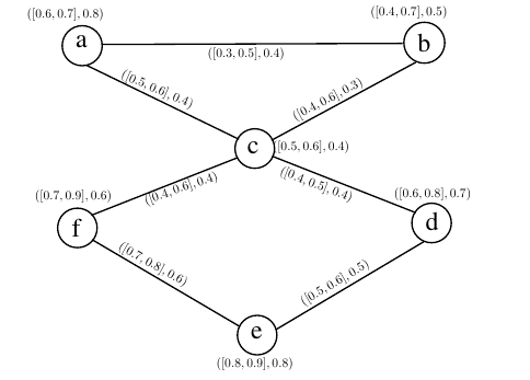
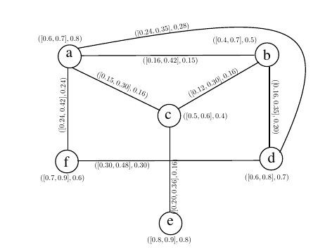
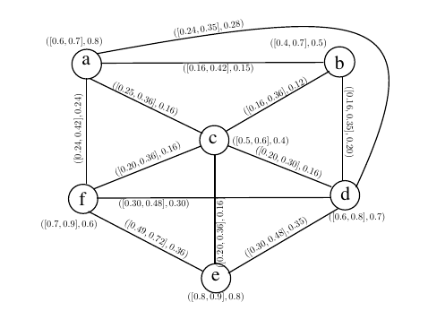
Example 5. Consider a cubic FG \({G}=(\mathcal{C}, \mathcal{D})\) on set of vertices \(\mathcal{V}=\{a,b,c,d,e,f\}\) as shown in Figure 4. The degree of memberships of the vertices and edges are taken arbitrarily as described in Figure 1. The cubic fuzzy open-neighbourhood and cubic fuzzy closed-neighbourhood are shown in Table 2:
| \(x\) | \(\mathcal{N}(t)\) | \(\mathcal{N}[t]\) |
| a | {(b,[0.3,0.5],0.4),(c,[0.5,0.6],0.4)} | {(b,[0.3,0.5],0.4),(c,[0.5,0.6],0.4)}\(\cup\){(a,[0.6,0.7],0.8)} |
| b | {(a,[0.3,0.5],0.4),(c,[0.4,0.6],0.3)} | {(a,[0.3,0.5],0.4),(c,[0.4,0.6],0.3)} \(\cup\){(b,[0.4,0.7],0.5)} |
| c | {(d,[0.4,0.5],0.4),(f,[0.4,0.6],0.4), | {(d,[0.4,0.5],0.4),(f,[0.4,0.6],0.4),(a,[0.5,0.6],0.4), |
| (a,[0.5,0.6],0.4),(b,[0.4,0.6],0.3)} | (b,[0.4,0.6],0.3)} \(\cup\) {(c,[0.5,0.6],0.4)} | |
| d | {(c,[0.4,0.5],0.4),(e,[0.5,0.6],0.5)} | {(c,[0.4,0.5],0.4),(e,[0.5,0.6],0.5)}\(\cup\){(d,[0.6,0.8],0.7)} |
| e | {(d,[0.5,0.6],0.5),(f,[0.7,0.8],0.6)} | {(d,[0.5,0.6],0.5),(f,[0.7,0.8],0.6)}\(\cup\){(e,[0.8,0.9],0.8)} |
| f | {(c,[0.4,0.6],0.4),(e,[0.7,0.8],0.6)} | {{(c,[0.4,0.6],0.4),(e,[0.7,0.8],0.6)}\(\cup\){(f,[0.7,0.9],0.6)} |
The cubic fuzzy open-neighbourhood graph \(\mathcal{N}({G})\) in Figure 8 and the cubic fuzzy closed-neighbourhood graph \(\mathcal{N}[{G}]\) in Figure 9 of the cubic graph \({G}\) in Figure 10 are shown.
Definition 15. Let \({G}=(\mathcal{C}, \mathcal{D})\) be a cubic FG. The (open) (k)-neighbourhood graph of \({G}\) is a cubic FG \(\mathcal{N}_{(k)}({G})=(\mathcal{C}, \mathcal{D})\) with \(\mathcal{C}(\mathcal{N}_{(k)}({G})=\mathcal{C}({G})\) and \(\mathcal{D}(\mathcal{N}_{(k)}({G}))=\{(t,u);\mathcal{N}(t)\cap\mathcal{N}(u)>k\}\) and \(\mu_{\mathcal{D}}: \mathcal{V}\times \mathcal{V}\rightarrow [0,1]\times[0,1]\) and \(\lambda_{\mathcal{D}}: \mathcal{V}\times \mathcal{V}\rightarrow [0,1]\) such that:\[\begin{aligned} % \nonumber to remove numbering (before each equation) \mu^L_\mathcal{D}(t,u) &=& \frac{\check{k}-k}{k}[\mu^L_\mathcal{C}(t)\wedge\mu^L_\mathcal{C}(u)]h^L(\mathcal{N}(t)\cap\mathcal{N}(u))\\ \mu^U_\mathcal{D}{(t,u)} &=& \frac{\check{k}-k}{k}[\mu^U_\mathcal{C}(t)\wedge\mu^U_\mathcal{C}(u)]h^U(\mathcal{N}(t)\cap\mathcal{N}(u))\\ \lambda_{\mathcal{D}}{(t,u)} &=&\frac{\check{k}-k}{k}[\lambda_\mathcal{C}(t)\wedge\lambda_\mathcal{C}(u)]h(\mathcal{N}(t)\cap\mathcal{N}(u)), \end{aligned}\] where \(\check{k}=|\mathcal{N}(t)\cap\mathcal{N}(u)|.\)
Definition 16. Let \({G}=(\mathcal{C}, \mathcal{D})\) be a cubic FG. The cubic fuzzy (close) [k]-neighbourhood graph of \({G}\) is a cubic FG \(\mathcal{N}_{[k]}[{G}]=(\mathcal{C}, \mathcal{D})\) with \(\mathcal{C}(\mathcal{N}_{[k]}[{G}])=\mathcal{C}({G})\) and \(\mathcal{D}(\mathcal{N}_{[k]}[{G}])=\{(t,u);\mathcal{N}[t]\cap\mathcal{N}[u]>k\}\) and \(\mu_{\mathcal{D}}: \mathcal{V}\times \mathcal{V}\rightarrow [0,1]\times[0,1]\) and \(\lambda_{\mathcal{D}}: \mathcal{V}\times \mathcal{V}\rightarrow [0,1]\) such that: \[\begin{aligned} % \nonumber to remove numbering (before each equation) \mu^L_\mathcal{D}(t,u) &=& \frac{\check{k}-k}{k}[\mu^L_\mathcal{C}(t)\wedge\mu^L_\mathcal{C}(u)]h^L(\mathcal{N}[t]\cap\mathcal{N}[u])\\ \mu^U_\mathcal{D}{(t,u)} &=& \frac{\check{k}-k}{k}[\mu^U_\mathcal{C}(t)\wedge\mu^U_\mathcal{C}(u)]h^U(\mathcal{N}[t]\cap\mathcal{N}[u])\\ \lambda_{\mathcal{D}}{(t,u)} &=&\frac{\check{k}-k}{k}[\lambda_\mathcal{C}(t)\wedge\lambda_\mathcal{C}(u)]h(\mathcal{N}[t]\cap\mathcal{N}[u]), \end{aligned}\] where \(\check{k}=|\mathcal{N}[t]\cap\mathcal{N}[u]|.\)
Now we can proceed to a theorem that provides a significant property of p-competition cubic FGs.
Theorem 5. There exist one edge in \(\mathcal{N}[{G}]\) for every edge in a cubic graph \({G}.\)
Proof. Let edge \((t,u)\) be any edge of cubic graph \({{G}}=(\mathcal{C}, \mathcal{D}).\) Consider the corresponding cubic fuzzy closed-neighbourhood graph \(\mathcal{N}[{G}]=(\mathcal{C}, {\mathcal{D}}).\) Then \((t,u)\in \mathcal{N}[t]\) and \((t,u)\in \mathcal{N}[u].\) Thus \((t,u)\in \mathcal{N}[t]\cap\mathcal{N}[u].\) Hence, \(h^L(\mathcal{N}[t]\cap\mathcal{N}[u])\neq0,\) \(h^U(\mathcal{N}[t]\cap\mathcal{N}[u])\neq0\) and \(h(\mathcal{N}[t]\cap\mathcal{N}[u])\neq0.\) Therefore, \[\begin{aligned} % \nonumber to remove numbering (before each equation) \mu^L_\mathcal{D}(t,u) &=& \mu^L_\mathcal{C}(t)\wedge\mu^L_\mathcal{C}(u)h^L(\mathcal{N}[t]\cap\mathcal{N}[u])\neq0,\\ \mu^U_\mathcal{D}{(t,u)} &=& \mu^U_\mathcal{C}(t)\wedge\mu^U_\mathcal{C}(u)h^U(\mathcal{N}[t]\cap\mathcal{N}[u])\neq0,\\ \lambda_{\mathcal{D}}{(t,u)} &=&\lambda_\mathcal{C}(t)\wedge\lambda_\mathcal{C}(u)h(\mathcal{N}[t]\cap\mathcal{N}[u])\neq0. \end{aligned}\] So for every \((t,u)\) in \({G},\) there is \((t,u)\) in \(\mathcal{N}[{G}].\) ◻
In this section, the m-step cubic fuzzy digraph \(\mathcal{S}(\vec{{G}}_m)\), which forms the foundation for constructing m-step cubic fuzzy CMGs has been introduced. The m-step digraph considers paths of length m between vertices, thereby capturing the indirect relationships that might not be apparent in a single step. This concept is crucial as it allows us to analyze the structure of the graph beyond immediate connections, which can reveal deeper insights into the network’s topology.
Definition 17. The m-step cubic fuzzy digraph \(\mathcal{S}(\vec{{G}}_m)\) of a CuDG \(\vec{{G}}=(\mathcal{C}, \mathcal{D})\) is indicated as \(\mathcal{S}(\vec{{G}}_m)=(\mathcal{C},\mathcal{D})\) with \(\mathcal{C}(\mathcal{S}(\vec{{G}_m}))=\mathcal{C}({G})\) and \(\mathcal{D}(\mathcal{S}(\vec{{G}_m}))=\{(t,u);\exists {\rm ~a ~CuDP~ of~ m~ length~ from}~ t~ to~ u, \vec{P}^m_{(t,u)} in~ \vec{{G}}\}.\)
This definition establishes the framework for constructing m-step cubic fuzzy CMGs by considering paths of length m between vertices. Next, the concept of cubic fuzzy m-step out and in neighborhoods of a vertex in a CuDG has been introduced. These neighborhoods consist of vertices that can be reached from a given vertex \(t\) within m steps, along with the associated fuzzy membership values. These neighborhoods provide a localized view of the network, allowing us to examine how a vertex is connected to others within a specified range, which is essential for understanding the influence and reach of a vertex within the graph.
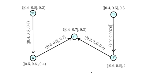
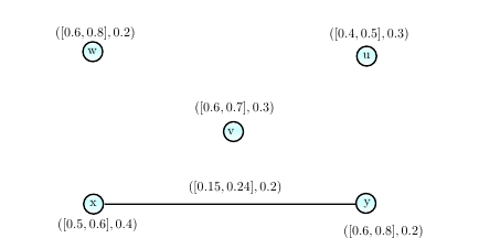
Example 6. An example of 2-step cubic fuzzy CMGs of the CuDG of Figure 11 is shown in Figure 12.
Definition 18. The cubic fuzzy m-step out neighbourhood of any vertex \(t\) of a CuDG \(\vec{{G}}=(\mathcal{C}, \mathcal{D})\) is CS \(\mathcal{N}^+_m(t)=(V^{+}_{t},r^{+}_t, s^{+}_t),\) where \[\label{3} V^{+}_{t}=\{u| ~\exists {\rm ~a ~CuDP~ of~ m~ length~ from~} t~ to~ u, \vec{P}^m_{(t,u)}\},\tag{3}\] such that \[r^{+}_t : V^{+}_{t}\rightarrow[0,1]\times[0,1]\] specified by \[r^{+}_t = \{[\min\mu^L_\mathcal{D}(t,u), \min\mu^U_\mathcal{D}(t,u)];(t,u) {\rm ~is~ an~ edge~ of} \vec{P}^m_{(t,u)}\}\] and \[s^{+}_t: V^{+}_{t}\rightarrow[0,1]\] specified by \[s^{+}_t =\{\min\lambda_{\mathcal{D}}(t,u);(t,u) {\rm ~is~ an~ edge~ of} \vec{P}^m_{(t,u)}\}.\]
Definition 19. The cubic fuzzy m-step in neighbourhood of any vertex \(t\) of a CuDG \(\vec{{G}}=(\mathcal{C}, \mathcal{D})\) is CS \(\mathcal{N}^-_m(t)=(V^{-}_{t},r^{-}_t, s^{-}_t),\) where \[\label{4} V^{-}_{t}=\{u|~ \exists {\rm ~a ~CuDP~ of~ m~ length~ from}~ t~ to~ u, \vec{P}^m_{(t,u)}\},\tag{4}\] such that \[r^{-}_t : V^{-}_{t}\rightarrow[0,1]\times[0,1]\] specified by \[r^{-}_t = \{[\min\mu^L_\mathcal{D}(t,u), \min\mu^U_\mathcal{D}(t,u)],(t,u)~ is~ an~ edge~ of ~\vec{P}^m_{(t,u)}\}\] and \[s^{-}_t: V^{-}_{t}\rightarrow[0,1]\] specified by \[s^{-}_t =\{\min\lambda_{\mathcal{D}}(t,u),(t,u)~ is~ an~ edge~ of~ \vec{P}^m_{(t,u)}\}.\]
The notion of an independent strong vertex, which is a vertex that maintains a high degree of membership across multiple m-step neighborhoods has also been explored. The strength of such a vertex is quantified using specific measures, which aggregate the membership values from all relevant connections.
Definition 20. Let \({G}=(\mathcal{C}, \mathcal{D})\) be a cubic graph. The m-step cubic fuzzy CMG of \({G}\) is indicated by \({G}_m=({C}, {D})\) with \(\mathcal{C}({G}_m)=\mathcal{C}({G})\) and \(\mathcal{D}({G}_m)=\{(t,u);\mathcal{N}(t)\cap\mathcal{N}(u) >k\}\) in cubic graph. The degree of membership of the edge \((t,u)\) are defined as: \[\begin{aligned} % \nonumber to remove numbering (before each equation) \mu^L_{D}(t,u) &=& (\mu^L_{C}(t)\wedge\mu^L_{C}(u))h^L(\mathcal{N}^+_m(t)\cap\mathcal{N}^+_m(u)),\\ \mu^U_{D}{(t,u)} &=& (\mu^U_{C}(t)\wedge\mu^U_{C}(u))h^U(\mathcal{N}^+_m(t)\cap\mathcal{N}^+_m(u)),\\ \lambda_{{D}}{(t,u)} &=&(\lambda_{C}(t)\wedge\lambda_{C}(u))h(\mathcal{N}^+_m(t)\cap\mathcal{N}^+_m(u)). \end{aligned}\]
Definition 21. Let \(\vec{{G}}=(\mathcal{C},
\mathcal{D})\) be a CuDG. Suppose \(u\) be the common vertex of m-step cubic
fuzzy out neighbourhoods of vertices \(t_1,
t_2,\ldots, t_n,\) \(n\) is a
positive integer. The m-step vertex \(u \in
V\) is called independent strong vertex if \(\mu^L_m(t,u)>0.5,\) \(\mu^U_m(t,u)>0.5\) and \(\lambda_m(t,u)>0.5,\) for all \(i=1,2,\ldots,n.\) Further, the strength of
this vertex \(u\) is denoted by \(\mathcal{S}_m(u)\) and is specified as:
\[\label{5}
\mathcal{S}(u)=([S^L_m(u),S^U_m(u)], S_m(u)),\tag{5}\] where \[S^L_m(u)=\frac{\sum\limits_{i=1}^{n}\mu^L_m(\overrightarrow{t_i,u})}{n},~~
S^U_m(u)=\frac{\sum\limits_{i=1}^{n}\mu^U_m(\overrightarrow{t_i,u})}{n},~~
S_m(u)=\frac{\sum\limits_{i=1}^{n}\lambda_m(\overrightarrow{t_i,u})}{n}.\]
This definition provides a measure of how strong a vertex \(u\) is within its m-step neighbourhood.
Theorem 6. If a vertex \(u\) is independent strong then \(S^L_m(u)>0,\) \(S^U_m(u)>0\) and \(S_m(u)>0.\)
Proof. Let \(\vec{{G}}=(\mathcal{C}, \mathcal{D})\) be a CuDG. Let \(u\) be the common vertex of m-step cubic fuzzy out neighbourhoods of vertices \(t_1, t_2,\ldots, t_n,\) \(n\) belong to positive integers. Since, the vertex \(u\) is independent strong as given so \(\mu^L_m(\overrightarrow{t_i,u})>0.5\) for all \(i=1,2,\ldots,n.\) Therefore, \[S^L_m(u)=\frac{\mu^L_m(\overrightarrow{t_1,u})+\mu^L_m(\overrightarrow{t_2,u})+\ldots+\mu^L_m(\overrightarrow{t_n,u})}{n} >\frac{0.5+0.5+\ldots+0.5}{n}=0.5,\] \[S^U_m(u)=\frac{\mu^U_m(\overrightarrow{t_1,u})+\mu^U_m(\overrightarrow{t_2,u})+\ldots+\mu^U_m(\overrightarrow{t_n,u})}{n} >\frac{0.5+0.5+\ldots+0.5}{n}=0.5,\] \[S_m(u)=\frac{\lambda_m(\overrightarrow{t_1,u})+\lambda_m(\overrightarrow{t_2,u})+\ldots+\lambda_m(\overrightarrow{t_n,u})}{n} >\frac{0.5+0.5+\ldots+0.5}{n}=0.5.\] ◻
Theorem 7. The edges of \(\mathcal{S}(\vec{{G}}_m)\) must also be independent strong if all of its vertices are.
Proof. Suppose that the CuDG \(\vec{{G}}=(\mathcal{C},
\mathcal{D})\) has independent strong vertices. Let \({G}_m =({C}, {D})\) be
a m-step cubic fuzzy CMG of \(\vec{{G}}.\) \[\label{6}
\mu^L_{D}(t,u)
=(\mu^L_{C}(t)\wedge\mu^L_{C}(u))h^L(\mathcal{N}_m(t)\cap\mathcal{N}_m(u),\tag{6}\]
if \(\mathcal{N}_m(t)\cap\mathcal{N}_m(u)\) is
empty then there doesn’t exists any edge among vertices \(t\) and \(u\) in \(\mathcal{N}_m({G}).\) If \(\mathcal{N}_m(t)\cap\mathcal{N}_m(u)\) is
non-empty then clearly \(h^L(\mathcal{N}^+_m(t)\cap\mathcal{N}^+_m(u))>
0.5\) as all the edges of \(\vec{{G}}\) must also be independent
strong hence, \[\label{7}
\mu^L_{D}(t,u)
=(\mu^L_{C}(t)\wedge\mu^L_{C}(u))h^L(\mathcal{N}^+_m(t)\cap\mathcal{N}^+_m(u))>\frac{1}{2}
(\mu^L_{C}(t)\wedge\mu^L_{C}(u)).\tag{7}\] In similar way,
we can show that \(\mu^U_{D}(t,u)>\frac{1}{2}
(\mu^U_{C}(t)\wedge\mu^U_{C}(u))\) and \(\lambda_{D}(t,u)>\frac{1}{2}
(\lambda_{C}(t)\wedge\lambda_{C}(u)).\)
This suggests that each and every edge of \(\mathcal{S}(\vec{{G}}_m)\) is
independently strong. ◻
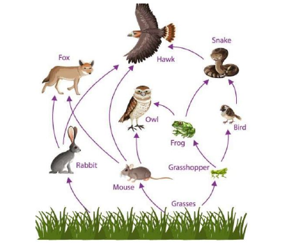
In this Section, an application of cubic fuzzy CMGs. Relationships among predators and prey, in which one organism (the predator) pursues, captures, and consumes another organism (the prey) for food, are a basic component of ecological interactions has been discussed. These connections are essential for keeping ecosystems in balance. Take the cubic fuzzy food chain of animals as an example: Grasses, Rabbit, Mouse, Grasshopper,Grain, Bird, Frog, Snake, Fox, Owl and Hawk as shown in Figure 13.
The goal is to find those species which have strong competition among them by using CMGs. The interval degree of belongingness of each species characterizes strong access to itself requirements in particular duration of time while simple fuzzy membership indicates their present requirements from environment. The cubic fuzzy food web is shown in Figure 14.
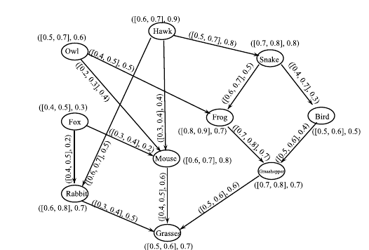
Cubic fuzzy CMG can be constructed to investigate the strength of competition between species having common food prey. The Cubic fuzzy out neighbourhoods are given in table 3.
| Species | Cubic fuzzy out neighbourhoods of each specie |
| Hawk | {(Rabbit,[0.6,0.7],0.5),(Snake,[0.5,0.7],0.8)} |
| Rabbit | {(Grasses,[0.3,0.4],0.5)} |
| Bird | {(Grasshopper,[0.5,0.6],0.4)} |
| Grasshopper | {(Grasses,[0.5,0.6],0.6)} |
| Mouse | {(Grasses,[0.4,0.5],0.6)} |
| Snake | {(Frog,[0.6,0.7],0.5),(Bird,[0.4,0.7],0.3)} |
| Frog | {(Grasshopper,[0.7,0.8],0.7)} |
| Fox | {(Rabbit,[0.4,0.5],0.2),(Mouse,[0.3,0.4],0.2)} |
| Owl | {(Mouse,[0.2,0.3],0.4),(Frog,[0.4,0.5],0.5)} |
Hawks are predatory birds known for their excellent vision and
hunting abilities. They prey on small animals, including mouse, rabbit
snake and birds. Hawks use their sharp talons and beaks to catch and
kill mice, which serve as their primary food source.The degree of
belongingness \(([0.6, 0.7],0.9)\),
which shows that Hawk was \(60\% –
70\%\) strong in accessing to itself requirements in past and
\(90\%\) strong in its present
requirements from environment. The edge from Hawk to Snake shows degree
of belongingness \(([0.5, 0.7],0.6)\)
represent that the Lion is \(50\% –
70\%\) predominated on Snake in past environment and \(60\%\) predominated on Snake in present
environment.
The cubic fuzzy CMG is shown in Figure 15.
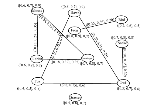
The edge membership values between two species represent the degree dominated on common food. According to Figure 14, there is a strong competition between Hawk and Snake common food. CMG can be constructed to investigate the strength of competition between species common food prey.
The paper examines the idea of cubic fuzzy CMGs, its variations and
uses. The concept of cubic fuzzy out neighbourhoods and in
neighbourhoods is introduced in order to use CSs to describe
relationships in a graph. Following that, the study describes various
varieties of cubic fuzzy competitive graphs based on external
neighbourhoods, including cubic fuzzy k-competitive graphs,
p-competitive cubic FGs, and m-step cubic fuzzy CMGs. To shed further
light on graph interactions and competition, the varieties of cubic FGs
including open and closed neighbourhood cubic FGs, cubic fuzzy (k)(open)
neighbourhood graphs, and cubic fuzzy [k](close) neighbourhood graphs
are also introduced.These cubic fuzzy CMGs are further categorized into
three specific types: cubic fuzzy \(k\)-competition graphs, which depict
competition at the \(k\)th order
between components; \(p\)-competition
cubic fuzzy graphs, which focus on competition based on membership
degrees; and \(m\)-step cubic fuzzy
competition graphs, which explore competition in terms of steps.
Additionally, several theorems and conditions concerning independent
strong vertices and edges are validated for these cubic fuzzy
competition graph classes. To show how rivalry between predators and
prey affects each other over time, a cubic fuzzy CMG application in
predator-prey dynamics is employed.
It is expected that in future this work can be extended to cubic fuzzy
CMGs, including cubic fuzzy intuitionistic CMGs and cubic fuzzy
Pythagorean CMGs, and some interesting properties along with
applications can be obtained.
This research is partially supported by the Higher Education Commission of Pakistan under the HEC-NRPU project No.14567.
There is no conflict of interest related to this work.