
Let \(G\) be a graph with vertices \(V(G)\) and edges \(E(G)\); we assume that all graphs are simple, undirected, and connected. For notation, we let \(n = |V(G)|\), \(m = |E(G)|\), \(deg(v) = |\{ab \in E(G) : v \in \{a,b\}\}|\), \(\delta(G) = \min_{v \in V(G)}deg(v)\), and \(\Delta(G) = \max_{v \in V(G)}deg(v)\). The open-neighborhood of a vertex \(v \in V(G)\), denoted \(N(v)\), is the set of all vertices adjacent to \(v\): \(\{w \in V(G) : vw \in E(G)\}\). The closed-neighborhood of a vertex \(v \in V(G)\), denoted \(N[v]\), is the set of all vertices adjacent to \(v\), as well as \(v\) itself: \(N(v) \cup \{v\}\). A vertex set \(S \subseteq V(G)\) is a (closed) dominating set if all vertices are within the closed neighborhood of some \(v \in S\); that is, \(\cup_{v \in S}{N[v]} = V(G)\). Similarly, \(S \subseteq V(G)\) is an open-dominating set if all vertices are within the open neighborhood of some \(v \in S\); that is, \(\cup_{v \in S}{N(v)} = V(G)\).
Assume that \(G\) models a facility with a possible “intruder” (or a multiprocessor network with a possible malfunctioning processor), where we want to be able to precisely determine the location of the intruder by placing (the minimum number of) detectors. Much work has been done on the topic of the graphical parameters involving various types of detectors. If a detector at \(v\) can determine only whether or not the intruder is in \(N[v]\), then the detection system is called an identifying code (IC) as introduced by Karpovsky, Charkrabarty and Levitin [16]. A dominating set \(S\) of \(V(G)\) is an identifying code if for any any two distinct vertices \(u,v \in V(G)\), we have \(N[u] \cap S \neq N[v] \cap S\). If a detector at \(v\) can determine only whether or not the intruder is in \(N[v]\) but can differentiate \(v\) from \(N(v)\), then the detection system is called a locating-dominating (LD) set, as introduced in Slater [25]. A dominating set \(S\) of \(V(G)\) is a locating-dominating set if for any two distinct vertices \(u,v \in V(G) – S\), we have \(N(u) \cap S \neq N(v) \cap S\).
This paper focuses on a detection system where a sensor at vertex \(v\) can sense intruders at adjacent vertices (i.e., within \(N(v)\)), but not at \(v\) itself. This type of detection system is called an open-locating-dominating (OLD) set, as introduced by Honkala, Laihonen and Ranto [11] and Seo and Slater [21]. An open-dominating set \(S \subseteq V(G)\) is an open-locating-dominating set if for any two distinct vertices \(u,v \in V(G)\), we have \(N(u) \cap S \neq N(v) \cap S\). Additional recent work on variations of OLD sets with larger detection ranges includes Givens et al. [9]. Jean and Lobstein [12] have maintained a bibliography, currently with more than 500 entries, for work on detection system related topics.
For an OLD set \(S \subseteq V(G)\) and \(u \in V(G)\), we let \(N_S(u) = N(u) \cap S\) denote the (open) dominators of \(u\) and \(dom(u) = |N_S(u)|\) denote the (open) domination number of \(u\). A vertex \(v \in V(G)\) is \(k\)-open-dominated by an open-dominating set \(S\) if \(|N_S(v)| \ge k\). If \(S\) is an open-dominating set and \(u,v \in V(G)\), \(u\) and \(v\) are \(k\)-distinguished if \(|N_S(u) \triangle N_S(v)| \ge k\), where \(\triangle\) denotes the symmetric difference. If \(S\) is an open-dominating set and \(u,v \in V(G)\), \(u\) and \(v\) are \(k^\#\)-distinguished if \(|N_S(u) – N_S(v)| \ge k\) or \(|N_S(v) – N_S(u)| \ge k\).
The purpose of \(k\)-domination in a detection system is to guarantee there are at least \(k\) detectors monitoring each location in the graph simultaneously, which can allow for a level of basic fault tolerance. A fault-tolerant variant of an OLD set is called a redundant open-locating-dominating (RED:OLD) set which is resilient to a (single) detector being destroyed or going offline [23]. That is, an OLD set \(S \subseteq V(G)\) is a RED:OLD set if \(\forall v \in S\), \(S – \{v\}\) is an OLD set. For fault-tolerance beyond simple \(k\)-redundancy, we conceptually establish that all detectors transmit either \(0\) to represent the absence of an intruder, or \(1\) to represent the presence of an intruder. A false negative is therefore when a detector incorrectly transmits a \(0\) instead of a \(1\), while a false positive is when a detector incorrectly transmits a \(1\) instead of a \(0\). An OLD set is called an error-detecting open-locating-dominating (DET:OLD) set if it can tolerant any single false negative [23]. Extending this, an OLD set is called an error-correcting open-locating-dominating (ERR:OLD) set, if it can tolerate any single false positive. The following theorem characterizes OLD, RED:OLD, DET:OLD, and ERR:OLD sets and they are useful in constructing those sets or verifying whether a given set meets their requirements.
(i) an OLD set if and only if every pair of vertices is 1-distinguished [14];
(ii) a RED:OLD set if and only if all vertices are 2-dominated and all pairs are 2-distinguished [23];
(iii) a DET:OLD set if and only if all vertices are 2-dominated and all pairs are \(2^\#{}\)-distinguished [23];
(iv) an ERR:OLD set if and only if all vertices are 3-dominated an all pairs are 3-distinguished.
In this paper, we will focus on the ERR:OLD parameter. As can be seen in Theorem 1.1, each new fault-tolerant capability on top of the basic OLD set demands stronger requirements for both the domination and distinguishing properties of the detector set. To see why the requirements for DET:OLD are not sufficient for ERR:OLD, consider the following two simple examples using detector set \(S \subseteq V(G)\). Firstly, if there is some 2-dominated vertex \(v\), with \(N_S(v) = \{p,q\}\), then an intruder at \(v\) coupled with a false-negative at \(p\) is indistinguishable from the absence of an intruder at \(v\) coupled with a false-positive at \(q\). Thus, 2-domination is insufficient for an ERR:OLD set. And secondly, if there are two vertices \(u,v\) with \(N_S(u) \cap N_S(v) = \{a,b\}\) and \((u,v)\) are \(2^{\#}\)-distinguished with \(N_S(v)-N_S(u) = \{p,q\}\), then \((p,q,a,b)\) transmitting \((0,1,1,1)\) could be due to a false-positive at \(q\) (in which case the intruder is at \(u\)) or a false-negative at \(p\) (in which case the intruder is at \(v\)). Thus, we cannot eliminate either of \(u\) or \(v\) as the intruder location, meaning \(2^\#\)-distinguishing is insufficient for an ERR:OLD. Indeed, it has been shown that an ERR:OLD set, or rather an equivalent error-correcting separating set, requires 3-domination and 3-distinguishing [24]. With both of these stronger properties, we see that two previous problem cases are resolved.
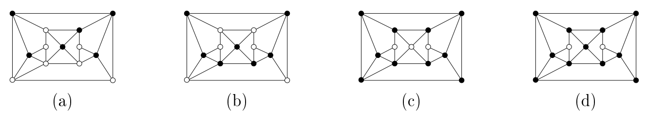
For finite graphs, the notations \(\textrm{OLD}(G)\), \(\textrm{RED:OLD}(G)\), \(\textrm{DET:OLD}(G)\), and ERR: OLD(G) represent the cardinality of the smallest possible OLD, RED:OLD, DET: OLD, and ERR:OLD sets on graph \(G\), respectively [23]. From Figure 1, which shows optimal solutions on the given graph which we will call \(G\), we see that \(\textrm{OLD}(G) = 6\), \(\textrm{RED:OLD}(G) = 7\), \(\textrm{DET:OLD}(G) = 10\), and \(\textrm{ERR:OLD}(G) = 11\).
In Section 2, we characterize the existence criteria for error-correcting open-locating-dominating sets in an arbitrary graph. We also consider extremal graphs that require every vertex to be a detector. In Section 3, we present a proof that the problem of finding a minimum error-correcting open-locating-dominating set in an arbitrary graph is NP-complete. We conclude with Section 4 by establishing bounds on the minimum densities of error-correcting open-locating-dominating sets on the infinite square grid, infinite triangular grid, and infinite king grid.
In this section, we discuss the existence criteria of ERR:OLD sets and some extremal graphs. But before this, we will first present previous results on the existence criteria and some extremal graphs for the OLD, RED:OLD, and DET:OLD parameters. From Theorem 1.1, it is not hard to see the following relationships between the minimum cardinality of the four fault-tolerant OLD sets:
From Theorem 1.1, by using \(S = V(G)\) we can arrive at the following existence criteria for OLD on arbitrary graphs:
Chellali et al. [2] proved the upper and lower bounds for \(\textrm{OLD}(G)\) on arbitrary graphs:
The upper bound of \(\textrm{OLD}(G) = n\) is achievable, and Foucaud et al. [7] later provided a full characterization for this class of extremal graphs:
Seo and Slater established the existence criteria for trees, determined the lower and upper bounds for \(\textrm{OLD}(G)\) on trees, and fully characterized the extremal trees which achieve these upper and lower bounds [22].
Henning and Yeo [10] determined the upper bound on OLD(G) when G is a cubic graph.
From Theorem 1.1, by using \(S = V(G)\), we can arrive at the following existence criteria for RED:OLD on arbitrary graphs:
These existence criteria can be simplified when discussing regular graphs:
Further, we have the following results from Seo [20] when discussing cubic graphs specifically:
Seo [20] has also constructed an infinite family of finite cubic graphs exhibiting the extremal value of \(\textrm{RED:OLD}(G) = \frac{2}{3}n\).
Similar to the existence criteria for OLD and RED:OLD sets, one can simply use Theorem 1.1 with \(S = V(G)\) to arrive at the existence criteria for DET:OLD sets in arbitrary graphs. While there are no simpler existence criteria on arbitrary graphs, the following necessary conditions have been found:
Further, we have the following results from Seo [20] when discussing cubic graphs specifically:
The lower bound from Theorem 2.17 is achieved by the infinite hexagonal grid [23] and an infinite family of finite cubic graphs [20].
Because an ERR:OLD set requires 3-domination, many graphs do not allow an ERR:OLD set to exist. In light of this, our next theorem characterizes all graphs that permit an ERR:OLD set.
Proof. First, assume to the contrary that there exists a vertex \(v\) with \(deg(v) \le 2\); then, \(v\) cannot be 3-dominated, a contradiction. Similarly, if we assume there exists \(a,c \in V(G)\) with \(|N(a) \triangle N(c)| \le 2\), then \(a\) and \(c\) could not be \(3\)-distinguished, a contradiction.
For the converse, suppose \(G\) satisfies both properties of the theorem statement. To demonstrate the existence of ERR:OLD, we will conservatively let \(S = V(G)\) be the detector set. Clearly, \(\delta(G) \ge 3\) guarantees all vertices will be 3-dominated, so we need only show that all vertex pairs are \(3\)-distinguished. Let \(u,v \in V(G)\) with \(u \neq v\). If \(d(u,v) \ge 3\) then \(u\) and \(v\) will have non-intersecting neighborhoods and thus be \(3\)-distinguished; otherwise, we can assume \(d(u, v) \le 2\). Suppose \(d(u, v) = 2\), and let \(uxv\) be a path from \(u\) to \(v\). If \(|N(u) \cap N(v)| = 1\), then \(u\) and \(v\) must be 4-distinguished, and we would be done, so assume \(\{x,y\} \subseteq N(u) \cap N(v)\) with \(x \neq y\). Then we have a \(C_4\) subgraph, \(uxvy\), so by hypothesis \(|N(u) \triangle N(v)| \ge 3\) and \((u, v)\) are \(3\)-distinguished. Finally, suppose \(d(u, v) = 1\). If there is some \(p \in (N(u) \triangle N(v)) – \{u,v\}\), then \(u\) and \(v\) will be 3-distinguished by \(\{u,v,p\}\), and we would be done; otherwise, we assume that \(N(u) \triangle N(v) = \{u,v\}\). Because \(\delta(G) \ge 3\), it must be that \(\exists p,q \in N(u) \cap N(v)\) with \(p \neq q\). Then we have a \(C_4\) subgraph \(upvq\), so by hypothesis \(u\) and \(v\) must be \(3\)-distinguished, completing the proof. ◻
From Theorem 2.18, it is clear that checking whether or not a graph permits an ERR:OLD set can be done in polynomial time.
Two distinct vertices \(u,v \in V(G)\) are said to be twins if \(N[u] = N[v]\) (closed twins) or \(N(u) = N(v)\) (open twins). From Theorem 2.18, we see that if \(G\) has twins \(u\) and \(v\), then it cannot have an ERR:OLD set since \(deg(u) = deg(v) \le 2\) or \(u\) and \(v\) form the corners of a \(C_4\) subgraph with \(|N(u) \triangle N(v)| \le 2\).
Next, we will show that there are no graphs with ERR:OLD sets on \(n \le 6\) vertices.
Proof. Firstly, we know that \(G\) cannot be acyclic because an ERR:OLD set requires \(\delta(G) \ge 3\). Thus, \(G\) has a cycle, which we will exploit in casing. We will proceed by casing on the size of the smallest cycle, which implies that edges cannot be added between the vertices of said smallest cycle. We assume \(n \le 6\), as otherwise we would be done. If the smallest cycle is \(C_k\) for \(5 \le k \le 6\), then every vertex in the cycle must have a third dominator, and these additional \(k\) vertices must all be distinct to avoid creating smaller cycles; thus \(n \ge 2k \ge 10 > 6\), a contradiction. Suppose the smallest cycle is a \(C_4\) subgraph \(abcd\), then each vertex in the cycle must have a third dominator, \(a’\), \(b’\), \(c’\), and \(d’\) adjacent to \(a\), \(b\), \(c\), and \(d\), respectively. We see that \(a’ \neq b’ \neq c’ \neq d’ \neq a’\); however, because \(n \le 6\) it must be that \(a’ = c’\) and \(b’ = d’\). We see that \(a\) and \(c\) cannot have any additional edges without creating a smaller cycle, but they are open twins and so cannot be \(3\)-distinguished, a contradiction. Thus, we can assume that \(G\) has a triangle.
Next, suppose there exists a 4-Cycle \(abcd\) with \(bd \in E(G)\), which we call a “diamond” subgraph. If \(ac \notin E(G)\) then distinguishing \(a\) and \(c\) will result in \(n \ge 7\), a contradiction; thus, we can assume that \(ac \in E(G)\), meaning we have a \(K_4\) subgraph. By symmetry, we can assume that \(a\), \(b\), and \(c\) have third dominators \(a’\), \(b’\), and \(c’\). If \(a’\), \(b’\), and \(c’\) are all distinct, then \(n \ge 7\) and we would be done; otherwise without loss of generality assume \(a’ = b’\). Suppose \(a’ = b’ = c’\); then we require \(da’ \in E(G)\) to be able to distinguish \(d\) and \(a’\), and by symmetry we have \(\exists x \in N(d) – N(a’) – \{a,b,c,d,a’\}\). We now have a \(K_5\) subgraph plus an extra vertex \(x \in N(d)\). Distinguishing \(a\) and \(b\) requires without loss of generality \(x \in N(a)\), but then \(a\) and \(d\) cannot be \(3\)-distinguished, a contradiction. Otherwise, we can assume \(a’ = b’ \neq c’\); we see that distinguishing \(a\) and \(b\) requires, without loss of generality, \(bc’ \in E(G)\). If \(a’d \in E(G)\) then \(dc’ \in E(G)\) to distinguish \(a\) and \(d\); however, \(b\) and \(d\) can no longer be \(3\)-distinguished, a contradiction, so we assume \(a’d \notin E(G)\) and \(dc’ \notin E(G)\). If \(a’c \in E(G)\) then \(b\) and \(c\) cannot be \(3\)-distinguished, a contradiction, so by symmetry we assume \(a’c \notin E(G)\) and \(c’a \notin E(G)\). Thus, 3-dominating \(a’\) and \(c’\) requires \(a’c’ \in E(G)\), but then \(c\) and \(a’\) cannot be \(3\)-distinguished, a contradiction. Thus, the existence of a diamond subgraph implies that \(n \ge 7\).
At this point, we know that \(G\) has a triangle, say \(abc\). To 3-dominate the vertices in \(abc\), assume \(\exists a’ \in N(a)-\{b,c\}\), \(\exists b’ \in N(b)=\{a,c\}\), and \(c’ \in N(c)-\{a,b\}\). Additionally, we can assume \(a’\), \(b’\), and \(c’\) are distinct because otherwise we produce a diamond subgraph. To 3-dominate \(a’\), \(b’\), and \(c’\) without producing a diamond subgraph, it must be that \(\{a’b’, b’c’, c’a’\} \subseteq E(G)\). At this point we can no longer add any edges without producing a diamond subgraph, but \(a’\) and \(b\) are not \(3\)-distinguished, a contradiction, completing the proof. ◻
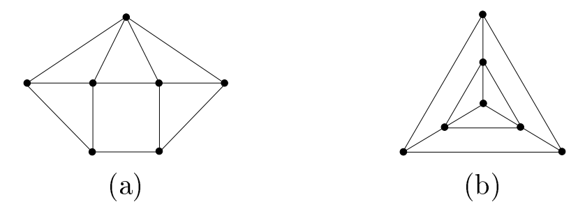
Figure 2 shows the first graphs with an ERR:OLD set in the lexicographic ordering of \((n,m)\) tuples; i.e., the graphs with the smallest number of edges given the smallest number of vertices. For ERR:OLD, this is \(n = 7\) and \(m = 12\).
Next, we will show the relation between the existence of ERR:OLD sets and DET:OLD sets for regular graphs.
Proof. Suppose \(|A – B| = k\). Then \(|A \cap B| = |A| – k = |B| – k\). Therefore \(|A \triangle B| = |A – B| + |B – A| = k + (|B| – |B \cap A|) = k + (|B| – (|B| – k)) = k + k\), completing the proof. ◻
Suppose \(G\) is a regular graph with DET:OLD. We can conservatively let \(S = V(G)\) be the set of detectors. Then every vertex pair in \(G\) must be \(2^{\#}\)-distinguished; thus, Theorem 2.22 yields that every vertex pair is \(4\)-distinguished, which is sufficient for the distinguishing requirement of ERR:OLD.
A graph is cubic or 3-regular if every vertex is of degree 3. Jean and Seo [13] have previously proven that a cubic graph has a DET:OLD set if and only if the graph is \(C_4\)-free; thus, we have the following existence criteria.
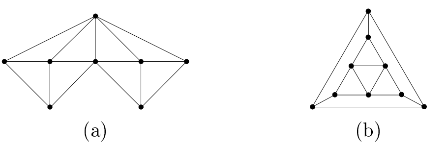
Now we consider extremal graphs with \(\textrm{ERR:OLD}(G) = n\) with least \(m\). If a graph \(G\) has an ERR:OLD set, then Theorem 2.18 yields that \(\delta(G) \ge 3\), which serves as a lower bound for the least \(m\), namely \(m \ge \frac{3n}{2}\). Figures 2 and 3 show extremal graphs with \(\textrm{ERR:OLD}(G) = n\) with the fewest number of edges when \(7 \le n \le 9\). For even \(n \ge 10\), we will show that cubic graphs exist which meet the theoretical lower bound of \(m = \frac{3n}{2}\). For odd \(n \ge 11\), this bound of \(m = \frac{3n}{2}\) is trivially unobtainable, but we introduce a new class of “almost-cubic” graphs meeting the lower bound of \(m = \frac{3n + 1}{2}\). In either case, we provide an extremal graph for each \(n \ge 10\).
When \(n \ge 10\), cubic and quasi-cubic graphs together form the entire family of extremal graphs with \(\textrm{ERR:OLD}(G) = n\) which have the minimum number of edges for a given \(n\). If \(S\) is an ERR:OLD set, we know that \(v \in S\) if \(\exists w \in N(v)\) with \(deg(w) = 3\). Because every vertex in a cubic or quasi-cubic graph is adjacent to a degree-3 vertex, these classes or graphs require \(\textrm{RED:OLD}(G) = n\) if they permit ERR:OLD.
Proof. Suppose \(G\) has a \(C_4\) subgraph, \(abcd\). Because \(G\) is cubic or quasi-cubic, at most one vertex in \(abcd\) can be degree 4, and all others will be degree 3. By symmetry, assume \(deg(a)=deg(c)=3\). Then \(a\) and \(c\) cannot be 3-distinguished, implying \(G\) does not have ERR:OLD.
For the converse, suppose \(G\) does not have ERR:OLD. Because \(\delta(G) \ge 3\), we know that an ERR:OLD set not existing implies \(\exists u,v \in V(G)\) where \(u\) and \(v\) are not 3-distinguished. Regardless of whether or not \(uv \in E(G)\), we see the only way to have \(u\) and \(v\) not be 3-distinguished is by having \(|N(u) \cap N(v)| \ge 2\), which creates a \(C_4\) subgraph, completing the proof. ◻
Suppose we have a cubic graph \(G\) that permits an ERR:OLD set. Then, we can construct a quasi-cubic graph from \(G\) as shown in the next theorem.
Proof. By Theorem 2.26, we know that \(G\) is \(C_4\)-free and we need only show that \(G’\) is likewise \(C_4\)-free. Suppose for a contradiction that \(G’\) has a \(C_4\) subgraph; then due to \(G\) being \(C_4\)-free, the \(C_4\) subgraph must involve vertex \(x\), which is an endpoint of every new edge in \(G’\). By symmetry, we can reduce the problem to two possible cases: the \(C_4\) includes edges \(\{ax,xb\}\) or edges \(\{ax,xc\}\), and we will consider \(y \in V(G)\) to be the opposite vertex of \(x\) in the \(C_4\) subgraph. If we are in the \(\{ax,xb\}\) case, we see that any choice of \(y\) results in \(aby\) forming a triangle in \(G\), a contradiction. Otherwise, in the \(\{ax,xc\}\) case we see that \(y \neq b\) and \(y \neq d\) because \(ab,cd \notin E(G’)\), so \(y\) causes \(ab\) and \(cd\) to be the ends of a \(P_5\) subgraph in \(G\), a contradiction, completing the proof. ◻
It has been shown that determining many graphical parameters related to detection systems, such as the minimum cardinality of an IC, LD, or OLD set, are NP-complete problems on arbitrary graphs [1,3,4,21]. Similarly, the problems involving RED:OLD and DET:OLD parameters have been known to be NP-complete [5,13]. We will now prove that the problem of determining the smallest ERR:OLD set is also NP-complete. For additional information about NP-completeness, see Garey and Johnson [8].
INSTANCE: Let \(X\) be a set of \(N\) variables. Let \(\psi\) be a conjunction of \(M\) clauses, where each clause is a disjunction of three literals from distinct variables of \(X\).
QUESTION: Is there is an assignment of values to \(X\) such that \(\psi\) is true?
INSTANCE: A graph \(G\) and integer \(K\) with \(7 \le K \le |V(G)|\).
QUESTION: Is there an ERR:OLD set \(S\) with \(|S| \le K\)? Or equivalently, is ERR:OLD(\(G\)) \(\le K\)?
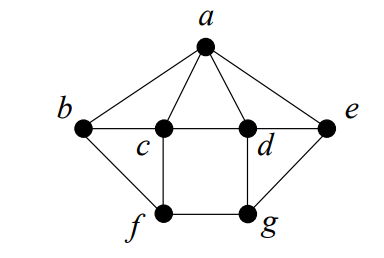
Proof. To 3-distinguish \(b\) and \(c\), we require \(\{b,c,d\} \subseteq S\). To 3-dominate \(b\), we additionally require \(\{a,f\} \subseteq S\). By symmetry, we have that \(V(G_{7}) \subseteq S\), completing the proof. ◻
Proof. Clearly, the ERR:OLD minimization is NP, as every possible candidate solution can be generated nondeterministically in polynomial time (specifically, \(O(n)\) time), and each candidate can be verified in polynomial time using Theorem 1.1 (iv). To complete the proof, we will now show a reduction from 3-SAT to ERR:OLD minimization.
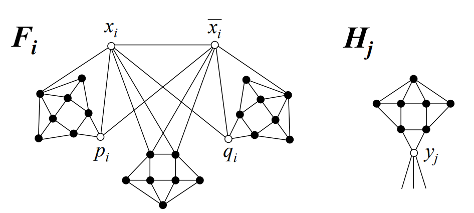
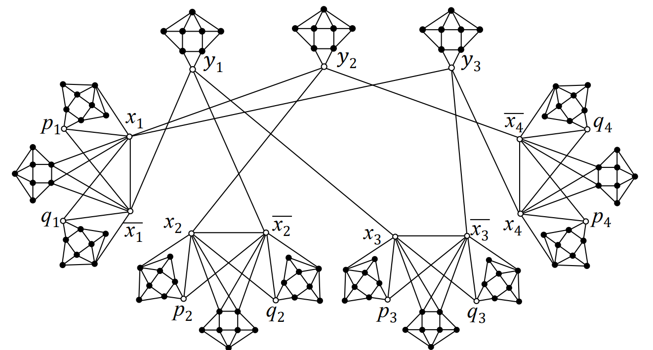
Let \(\psi\) be an instance of the 3-SAT problem with \(M\) clauses on \(N\) variables. We will construct a graph, \(G\), as follows. For each variable \(x_i\), create an instance of the \(F_i\) graph (Figure 5); this includes a vertex for \(x_i\) and its negation \(\overline{x_i}\). For each clause \(y_j\) of \(\psi\), create a new instance of the \(H_j\) graph (Figure 5). For each clause \(y_j = \alpha \lor \beta \lor \gamma\), create an edge from the \(y_j\) vertex to \(\alpha\), \(\beta\), and \(\gamma\) from the variable graphs, each of which is either some \(x_i\) or \(\overline{x_i}\); for an example, see Figure 6. The resulting graph has precisely \(25N + 8M\) vertices and \(51N + 17M\) edges, and can be constructed in polynomial time. To complete the problem instance, we define \(K = 22N + 7M\).
Suppose \(S \subseteq V(G)\) is an ERR:OLD set on \(G\) with \(|S| \le K\). By Lemma 3.1, we require at least all of the \(21N + 7M\) detectors shown by the shaded vertices in Figure 5. Additionally, in each \(F_i\) the vertices \(p_i\) and \(q_i\) require \(x_i \in S\) or \(\overline{x_i} \in S\) in order to be 3-dominated. Thus, we find that \(|S| \ge 22N + 7M = K\), implying that \(|S| = K\), so \(|\{x_i,\overline{x_i}\} \cap S| = 1\) for each \(i \in \{1, …, N \}\). For each \(H_j\), we see that \(y_j\) is not 3-dominated unless it is adjacent to at least one additional detector from its three neighbors in the \(F_i\) graphs; therefore, \(\psi\) is satisfiable.
For the converse, suppose we have a solution to the 3-SAT problem \(\psi\); we will show that there is a ERR:OLD, \(S\), on \(G\) with \(|S| \le K\). We construct \(S\) by first including all of the \(21N + 7M\) vertices as shown in Figure 5. Next, for each variable, \(x_i\), if \(x_i\) is true then we let the vertex \(x_i \in S\); otherwise, we let \(\overline{x_i} \in S\). Thus, the fully-constructed \(S\) has \(|S| = 22N + 7M = K\). It can be shown that every vertex pair is now 3-distinguished, and that every vertex which is not a \(y_j\) clause vertex is 3-dominated. Because we selected each \(x_i \in S\) or \(\overline{x_i} \in S\) based on a satisfying truth assignment for \(\psi\), each \(y_j\) must be adjacent to at least one additional detector vertex from the \(F_i\) graphs. Thus, all vertices are 3-dominated, implying \(S\) is an ERR:OLD set for \(G\) with \(|S| \le K\), completing the proof. ◻
In this section we will explore constructions of minimum-sized ERR:OLD sets on three popular infinite grids explored in literature: the infinite square grid (SQR), the infinite triangular grid (TRI), and the infinite king grid (KNG). Given this goal, a natural question is how we are to define such a “minimum-sized” infinite subset of an infinite vertex set. For this, we employ the concept of the density of a set of vertices and employ notations such as \(\textrm{ERR:OLD\%}(G)\) to denote the minimum density of an ERR:OLD set on \(G\), rather than the cardinality [23]. Formally, where \(B_r(v) = \{ u \in V(G) : d(u,v) \le r\}\), a subset \(S \subseteq V(G)\) on a locally-finite (i.e. \(B_r(v)\) finite for any finite \(r\)) (connected) graph \(G\) has density \(\limsup_{r \to \infty}{\frac{|B_r(v) \cap S|}{|B_r(v)|}}\) for any \(v \in V(G)\). Notably, the choice of center vertex \(v\) can affect the result of this calculation, in which case the density of the graph as a whole is not well-defined in practice. However, it has been proven that any graph satisfying the “slow-growth” property, \(\lim_{r \to \infty}\frac{|B_{r+1}(v)|}{|B_r(v)|} = 1\) for some \(v \in V(G)\), have the additional property that the density is invariant of the choice of center point [18].
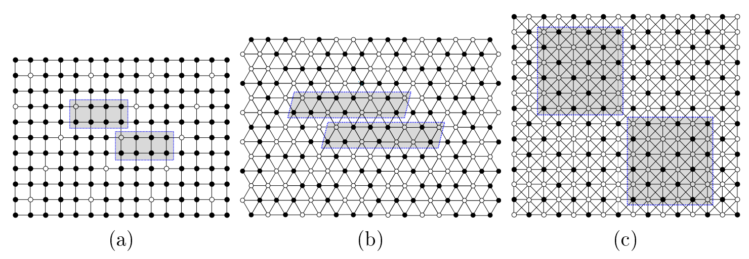
Figure 7 shows an ERR:OLD set with the minimum density we have found so far for the three infinite grids. One can verify that each of these ERR:OLD sets satisfies the domination and distinguishing requirements in Theorem 1.1. Figure 7 (a) shows an ERR:OLD set with a tiling of SQR where seven out of eight vertices are detectors, so \(\textrm{ERR:OLD\%}(SQR) \le \frac{7}{8}\). Similarly, we obtain \(\textrm{ERR:OLD\%}(TRI) \le \frac{4}{7}\) and \(\textrm{ERR:OLD\%}(KNG) \le \frac{4}{9}\) from Figure 7 (b) and (c), respectively.
To establish lower bound densities for domination-based parameters in infinite graphs, we employ a concept termed a share argument, originally introduced by Slater [26] and extensively utilized by other literature [14,19]. Essentially, this technique inverts the problem: instead of directly seeking a lower bound for the density of an ERR:OLD set, we determine an upper bound on the average share of a detector vertex \(v \in S\), denoted \(sh(v) = \sum_{u \in N(v)}{\frac{1}{dom(u)}}\), representing its total contribution to the domination of its neighbors. Because \(S\) is an open-dominating set, every vertex is 1-open-dominated, and each vertex with \(dom(u) = k\) contributes precisely \(\frac{1}{k}\) to the share of each of its \(k\) dominators, for a total of \(1\) per vertex in \(V(G)\). Therefore, an upper bound for the inverse average share of all detectors forms a lower bound for the density of \(S\) in \(V(G)\).
As an example of how share could be used to produce a lower bound for ERR:OLD, suppose \(G\) is \(k\)-regular and let \(v \in S\) be an arbitrary detector vertex in an ERR:OLD set \(S \subseteq V(G)\). We know that \(v\) has \(k\) neighbors and each neighbor must be 3-dominated due to \(S\) being an ERR:OLD set. Therefore, \(sh(v) \le \frac{1}{3} + \frac{1}{3} + … + \frac{1}{3} + \frac{1}{3} = \frac{k}{3}\). Because \(v\) was selected arbitrarily, this value of \(\frac{k}{3}\) serves as an upper bound for the average share of all detectors, and so its inverse, \(\frac{3}{k}\), represents a lower bound for the minimum density of an ERR:OLD in \(G\). Applying this finding to the infinite grids we will cover, we have the following naive lower bounds: \(\textrm{ERR:OLD\%}(SQR) \ge \frac{3}{4}\), \(\textrm{ERR:OLD\%}(TRI) \ge \frac{1}{2}\), and \(\textrm{ERR:OLD\%}(KNG) \ge \frac{3}{8}\).
In what follows, we will augment these same naive share arguments with a few additional pieces of information in order to arrive at much higher lower bounds. As a shorthand, we will let \(\sigma_A\) denote \(\sum_{k \in A}{\frac{1}{k}}\) for some sequence of single-character symbols, \(A\). Thus, \(\sigma_a = \frac{1}{a}\), \(\sigma_{ab} = \frac{1}{a} + \frac{1}{b}\), and so on.
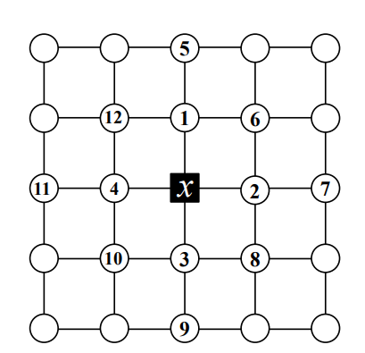
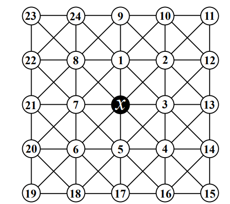
Proof. Let \(S\) be an ERR:OLD set on SQR and let \(x \in S\) be an arbitrary detector; we will use the labeling scheme shown in Figure 8. We see that in order to distinguish vertices \(v_1\) and \(v_2\) we require \(|\{v_5,v_7,v_8,v_{12}\}| \ge 3\). By symmetry, we also find that for any \(A \in \{ \{v_8,v_9,v_{11},v_{12}\}, \{v_5,v_6,v_{10},v_{11}\}, \{v_6,v_7,v_9,v_{10}\} \}\), \(|A \cap S| \ge 3\). Suppose \(v_6 \notin S\); then we require \(\{v_5,v_7,v_9,v_{10},v_{11}\} \subseteq S\) due to overlapping \(A\)-sets, as well as \(\{v_8,v_{12}\} \subseteq S\) to 3-dominate \(v_1\) and \(v_2\). Then \(sh(x) \le \sigma_{3344} = \frac{7}{6}\) and we would be done; otherwise, we can assume that \(v_6 \in S\) and by symmetry \(\{v_8,v_{10},v_{12}\} \subseteq S\) as well. Suppose \(v_5 \notin S\); then we also require \(\{v_7,v_{11}\} \subseteq S\) due to overlapping \(A\)-sets. Then \(sh(x) \le \sigma_{3344} = \frac{7}{6}\) and we would be done; otherwise, we can assume that \(v_5 \in S\) and by symmetry \(\{v_7,v_9,v_{11}\} \subseteq S\) as well. Then \(sh(x) \le \sigma_{4444} < \frac{7}{6}\), completing the proof. ◻
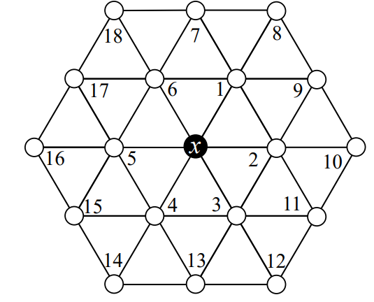
Proof. Let \(S\) be an ERR:OLD set on TRI and let \(x \in S\) be an arbitrary detector; we will use the labeling scheme shown in Figure 9. We know that every vertex must be 3-dominated; suppose \(\{v_1,v_3,v_5\}\) are all exactly 3-dominated. If \(v_2 \in S\), then we see that \(v_1\) and \(v_3\) (which are exactly 3-dominated) cannot be \(3\)-distinguished, a contradiction; otherwise we can assume that \(v_2 \notin S\) and by symmetry \(v_4,v_6 \notin S\) as well. Then to 3-dominated \(x\), we require \(\{v_1,v_3,v_5\} \subseteq S\). If at least two vertices in \(\{v_2,v_4,v_6\}\) are 4-dominated, then \(sh(x) \le \sigma_{344333} = \frac{11}{6}\) and we would be done; otherwise, without loss of generality assume that \(dom(v_2) = dom(v_4) = 3\). We see that \(v_6\) is already adjacent to three detectors, implying \(v_7 \notin S\), and by symmetry \(v_9 \notin S\) as well. Then \(v_1\) cannot be 3-dominated, a contradiction. Otherwise, we know that there must be at least one 4-dominated vertex in \(\{v_1,v_3,v_5\}\), and symmetry yields a second 4-dominated vertex in \(\{v_2,v_4,v_6\}\), giving \(sh(x) \le \sigma_{443333} = \frac{11}{6}\) and completing the proof. ◻
In order to simultaneously satisfy all four \(A\)-sets (“corners”), we require at least two vertices which are 4-dominated. There exists only one non-isomorphic configuration with the minimum of two such vertices, so without loss of generality let \(dom(v_1) \ge 4\) and \(dom(v_5) \ge 4\) with all other vertices in \(N(x)\) being (exactly) 3-dominated. Similar to before, we see that \(x \in N_S(v_2) \cap N_S(v_3)\), implying that \(\{v_1,v_{12},v_{13}\} \cap S = \varnothing\) and by symmetry \(\{v_5,v_{14},v_{20},v_{21},v_{22}\} \cap S = \varnothing\) as well. Applying the same reasoning to \(v_2\) and \(v_4\) gives us \(v_3 \notin S\), and by symmetry \(v_7 \notin S\) as well. Applying this again to \(v_2\) and \(v_8\) gives \(v_9 \notin S\), and by symmetry \(v_{17} \notin S\). To 3-dominate each vertex in \(\{v_2,v_3,v_4,v_6,v_7,v_8\}\), we require \(\{v_2,v_4,v_6,v_8,v_{10},v_{11},v_{15},v_{16},v_{18},v_{19},v_{23},v_{24}\} \subseteq S\). We see that \(dom(v_1) = dom(v_5) = 5\), so \(sh(x) = \sigma_{55333333} = \frac{12}{5}\) and we would be done. Otherwise, we know that there must be at least three vertices in \(N(x)\) which are 4-dominated. If \(N(x)\) has at least four vertices which are 4-dominated, then \(sh(x) \le \sigma_{44443333} < \frac{12}{5}\) and we would be done; otherwise, we may assume there are precisely three such vertices. Additionally, if any of these three vertices is 5-dominated, then \(sh(x) \le \sigma_{54433333} < \frac{12}{5}\) and we would be done; otherwise, we may assume \(N(x)\) contains exactly three vertices which are exactly 4-dominated, and all other vertices in \(N(x)\) are exactly 3-dominated. There are four non-isomorphic configurations which satisfy these constraints, as shown in Figure 11. We will now show that each of these cases has \(sh(x) \le \frac{12}{5}\).
Case 1: Suppose \(dom(v_1) = dom(v_4) = dom(v_6) = 4\) and all other vertices in \(N(x)\) are exactly 3-dominated. We first see that \(x \in N(v_3) \cap N(v_7)\), implying that \(\{v_1,v_5\} \cap S = \varnothing\). Applying this same logic to \(v_2\) and \(v_5\) gives us \(v_3 \notin S\), and by symmetry \(v_7 \notin S\) as well. Applying this to \(v_3\) and \(v_5\) gives us \(v_4 \notin S\), and \(v_6 \notin S\) by symmetry. We see that \(x\) cannot be 3-dominated, a contradiction, completing this case.
Case 2: Suppose \(dom(v_3) = dom(v_5) = dom(v_7) = 4\) and all other vertices in \(N(x)\) are exactly 3-dominated. Applying similar logic as before, from \(v_1\) and \(v_2\), we see that \(\{v_3,v_9,v_{10}\} \cap S = \varnothing\), and by symmetry \(\{v_7,v_{24}\} \cap S = \varnothing\) as well. Applying this to \(v_2\) and \(v_4\) gives us \(v_{13} \notin S\), and \(v_{21} \notin S\) by symmetry. Next, applying this to \(v_4\) and \(v_6\) gives us \(\{v_5,v_{17}\} \cap S = \varnothing\). Finally, applying this to \(v_2\) and \(v_8\) gives us \(v_1 \notin S\). To 3-dominated each vertex in \(\{v_1,v_2,v_8\}\), we require \(\{v_2,v_8,v_{11},v_{12},v_{22},v_{23}\} \subseteq S\). To distinguish \(v_1\) and \(x\), we require \(\{v_4,v_6\} \subseteq S\). Because \(v_3\) is now 4-dominated, it must be that \(v_{14} \notin S\), and \(v_{20} \notin S\) by symmetry. Then to 3-dominate \(v_4\) and \(v_6\) we require \(\{v_{15},v_{16},v_{18},v_{19}\} \subseteq S\). However, this causes \(v_5\) to be 5-dominated, a contradiction, completing this case.
Case 3: Suppose \(dom(v_2) = dom(v_5) = dom(v_7) = 4\) and all other vertices in \(N(x)\) are exactly 3-dominated. Applying the usual reasoning to \(v_3\) and \(v_4\) yields \(\{v_5,v_{13},v_{14}\} \cap S = \varnothing\), and by symmetry \(\{v_7,v_9,v_{24}\} \cap S = \varnothing\) as well. Applying this again to \(v_4\) and \(v_6\) gives \(v_{17} \notin S\), and by symmetry \(v_{21} \notin S\) as well. With \(v_1\) and \(v_4\), we have \(v_3 \notin S\), and by symmetry \(v_1 \notin S\) as well. With \(v_1\) and \(v_3\), we have \(v_2 \notin S\). To dominate each vertex in \(\{v_1,v_2,v_3,v_4,v_8\}\), we require \(\{v_4,v_8,v_{10},v_{11},v_{12},v_{15},v_{16},v_{22},v_{23}\} \subseteq S\). To 3-dominate \(x\), we require \(v_6 \in S\). Then \(v_5\) and \(v_7\) become 4-dominated, implying \(v_{18},v_{20} \notin S\), contradicting \(dom(v_6) = 3\) and completing this case.
Case 4: Suppose \(dom(v_1) = dom(v_2) = dom(v_5) = 4\) and all other vertices in \(N(x)\) are exactly 3-dominated. Applying the usual logic to \(v_3\) and \(v_4\) yields \(\{v_5,v_{13},v_{14}\} \cap S = \varnothing\). Applying this to \(v_6\) and \(v_7\) yields \(\{v_{20},v_{21}\} \cap S = \varnothing\). Vertices \(v_7\) and \(v_8\) yield \(\{v_1,v_{22}\} \cap S = \varnothing\). Vertices \(v_6\) and \(v_8\) yield \(v_7 \notin S\), and vertices \(v_4\) and \(v_6\) yield \(v_{17} \notin S\). To 3-dominate \(v_6\) and \(v_7\), we require \(\{v_6,v_8,v_{18},v_{19}\} \subseteq S\). If \(v_4 \in S\), then \(v_5\) would become 4-dominated, implying \(v_3,v_{16} \notin S\), contradicting that \(v_4\) is 3-dominated; otherwise, we may assume that \(v_4 \notin S\). To distinguish \(v_7\) and \(x\), we require \(v_2,v_3 \in S\). We see that \(v_1\) is 4-dominated, implying that \(\{v_9,v_{10},v_{24}\} \cap S = \varnothing\). Finally, we find that \(v_8\) cannot be 3-dominated, a contradiction, completing the proof. ◻
The following theorem summarizes bounds for minimum ERR:OLD set densities in three infinite grids: the infinite square grid (SQR), the infinite triangular grid (TRI), and the infinite king grid (KNG).
(i) For SQR, \(\frac{6}{7} \le \textrm{ERR:OLD\%}(SQR) \le \frac{7}{8}\).
(ii) For TRI, \(\frac{6}{11} \le \textrm{ERR:OLD\%}(TRI) \le \frac{4}{7}\).
(iii) For KNG, \(\frac{5}{12} \le \textrm{ERR:OLD\%}(KNG) \le \frac{4}{9}\).
Table 1 concludes this section with the upper and lower bounds for other fault-tolerant OLD sets on four of the most studied infinite grids including the infinite hexagonal grid (HEX). Note that \(\textrm{ERR:OLD\%}(\textrm{HEX}) = 1\) because HEX is cubic, which requires every vertex to be a detector.
| parameter | hexagonal | square | triangular | king |
| OLD [17,19,21] | \(\frac{1}{2}\) | \(\frac{2}{5}\) | \(\frac{4}{13}\) | \(\left[ \frac{6}{25}, \frac{1}{4} \right]\) |
| RED:OLD [15,23] | \(\frac{2}{3}\) | \(\frac{1}{2}\) | \(\frac{3}{8}\) | \(\left[ \frac{3}{10}, \frac{1}{3} \right]\) |
| DET:OLD [14,23] | \(\frac{6}{7}\) | \(\frac{3}{4}\) | \(\frac{1}{2}\) | \(\left[ \frac{3}{8}, \frac{13}{30} \right]\) |
| ERR:OLD | \(1\) | \(\left[ \frac{6}{7}, \frac{7}{8} \right]\) | \(\left[ \frac{6}{11}, \frac{4}{7} \right]\) | \(\left[ \frac{5}{12}, \frac{4}{9} \right]\) |
The authors declare no conflict of interest.