
Price volatility is the quantity of variability prices from the central price values of the security. It is the price swing of the security from the mean. Volatility is the amount of price fluctuation over specific period of time. Thus, volatility is often defined as high deviations from a global tendency [14]. Stock market volatility is one of the major challenges in financial markets, especially for portfolio managers, investors, traders and policy makers.
Volatility prediction is one of the crucial aspect of financial Mathematics, as it plays a key role in risk management, option pricing, investment decision, maximize return and portfolio optimization. All paricipants in the trading of S&P 500 stock price need to have better information about future price variation. Having this information is a challenging task that needs a demanding task.
The approach of machine learning algorithms has been growing to enhance the accuracy and reliability of stock market volatility forecasting [33].
Numerous models have been used in the prediction of stock price volatilities. They can be catagorized as parametric econometric, machine learning for time series and hybrid models. From the econometric models autoregressive conditional heteroskedasticity (ARCH) introduced by [9] describes the volatility at time \(t\) is correlated with the square of previous noise terms and generalized autoregressive conditional heteroskedasticity(GARCH) proposed by [4] explores that volatility at time \(t\) is obtained from the combination of the square of previous noise terms and the previous variance. Both ARCH and GARCH are symmetric to the sign of the noise. Exponential generalized autoregressive conditional heteroskedasticity (EGARCH) introduced by [26] and threhold generalized autoregressive conditional heteroskedasticity (TGARCH) proposed by [32] are the other asymmetric most common models. These econometric models have less volatility predictive powers.
Many researchers have made lot of efforts on forecasting volatility of securities by deep learning models for paramount information to optimal decision in financial markets.
Among the machine learning models recurrent neural network(RNN) especially Long Short term memory(LSTM) [11], convolutional neural networks (CNN) [6], Extreme gradient boosting(XGBoost) [7] and support vector machine(SVM) [30] are most frequently applied in the prediction of time series.
Some studies have shown that the performance of artificial neural network (ANN) is better than GARCH family models in volatility predictions since they can capture the non-linearity of the series and do not require the series to be stationary for modeling [28]. The combination of generalized autoregressive conditional heteroskedasticity family combined with deep learning hybrid models are the other price volatility forecasting models.
The hybrid model CNN-LSTM predicted the direction of stock market fluctuation better than many other models. This is, as CNN is good for extracting special local pattern features from the time series data and LSTM layers are good to capture long-term temporal dependencies, and hence CNN-LSTM can leverage the strength of both architectures for better performance [31,25,13,8,19].
On the other hand, hybrid of deep learning and GARCH-type models are usually found to have better prediction performances compared to single deep learning models or single econometric time series models [22]. The hybrid of convolutional neural network and Long Short term memory has a better forecast of volatility than the econometric GARCH models [29]. Their hybrid model improved the forecast of gold price volatility obtained by benchmark methods such as GARCH, support vector regression (SVR), ANN, ANN-GARCH, LSTM and CNN. Apart from the gold market, the effectiveness of hybrid models in forecasting the volatility of Copper was proved in the study of [12].
The combination of multi GARCH type models and the LSTM has better prediction performance in the stock price index volatility of COSPI 200 [18]. The hybrid model of EGARH and the feed forward artificial neural network demonstrated better volatility forecast in S&P500 return index [10]. The hybrid model of ARIMA GARCH and LSTM model outperformes the single alone models in the prediction of stock market time serie data [5].
The main focus of this paper is to analyze and compare the performance of econometric GARCH family models integrated with machine learning CNN and LSTM algorithms in the prediction of S&P 500 stock price volatility. To the best of our knowledge , this is the first idea to develop GARCH-CNN-LSTM in stock market volatility forecasting to improve the accuracy of the models. Furthermore, our investigation serves as a basis for further research in GARCH-deep learning hybrid models for volatility forecasting.
The remainder of this paper is organized as follows. Section 2 presents data description and methods on stock market volatility of S&P 500 using GARCH, CNN and LSTM hybrid models. Section 3 describes result and discussion. Finally, we provide conclusion of the study in Section 4.
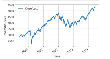
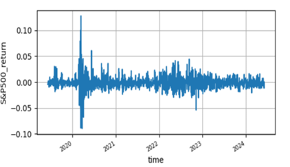
The historical stock price data of S&P 500 used in this study is extracted from Yahoo finance (GSPC) database that covers from 6 May 2019 to 6 May 2024 trading days. The time series plots of S&P 500 stock price is not stationary but its logarithmic return is stationary which are depicted in Figure 1 & Figure 2 . Furthermore this is justified using unit root test.
| ADF test critical values | |||||
| Variables | t-statistics | 1% | 5 % | 10 % | p-value |
| SP500 | -24.6854 | -3.4353 | -2.8636 | -2.5694 | 0.0000 |
From, Taable 1 clearly shows that the magnitude of S&P 500 stock return in t-statistics is greater than the magnitude at 5 % level which indicates that the return is stationary; thus, it is mean reverting.
| Mean | Max. | Min | Std.Dev | Skewness | Kurtosis | Jarque-Bera | P-value |
| 0.0005 | 0.08968 | -0.12765 | 0.01343 | -0.839736 | 17.501 | 11170.50 | 0.00000 |
From the descriptive statistics in Table 2, S&P 500 stock return has maximum and minimum values 0.089 and -0.1276 respectively which are highly deviated from the mean 0.0005. Moreover, the skewness and kurtosis of S&P 500 stock price return distiribution indicates negatively skewed and leptokurtic.
The value of Jarque-Bera in Table 2 is 11170 significantly greater than the p-value 0. Therefore, reject the null hypothesis(normality) and the distribution is not normally distributed.
| F-statistic | P-value | Obs*R-squared | P-value |
| 46.0142 | 0.0000 | 38.6794 | 0.0000 |
From Table 3 the LM – statistics of S&P 500 stock price return is 46.014 which is statistically significant. This shows that the null hypothesis (homoskedasticity) is rejected and reveals the presence of heteroskedasticity (time varying volatility). Therefore, GARCH family models are better fitting for forecasting the volatility of S&P 500 stock price .
The most frequently used model for forecasting the time varying variance is generalized autoregressive conditional heteroskedasticity model in which the variance of a time series is expressed as the combination of previous square shocks and the previous conditional variance. Mathematically: \[\label{eq1} \sigma^2_t=\alpha_0+\sum_{i=1}^{q}\alpha_i\varepsilon^2_{t-i}+\sum_{j=1}^{p}\beta_j\sigma^2_{t-j} ,\;\;\;\alpha_0>0,\alpha_i>0,q>0,p\geq 0 , \tag{1}\] when p=1 and q=1 ,it is called GARCH(1,1) and the conditional volatility of Eq. (1) becomes: \[\sigma^2_t=\alpha_0+\alpha_1\varepsilon^2_{t-1}+\beta_1\sigma^2_{t-1}. \tag{2}\]
The order of \(p\) and \(q\) is determined by partial autocorrelation function(PACF) in the square return. In most financial time-series, the GARCH (1,1) is superior to other higher order values of p and q [4,12].
This model is proposed by [26] to take into account the leverage effects of price fluctuation on conditional variance. This means that a negative shock (bad news) can have a greater impact on volatility than a positive shock(good news) of the same magnitude [21]. The conditional variance in EGARCH is given as:
\[log\sigma^2_t=\alpha_0+\sum_{i=1}^{p}\frac{\alpha_i\mid{\varepsilon_{t-i}\mid}}{\sigma_{t-i}}+\sum_{i=1}^{r}\frac{\gamma_i\varepsilon_{t-i}}{\sigma_{t-i}} +\sum_{j=1}^{q}\beta_jlog\sigma^2_{t-j}, \tag{3}\] where p, q and r are the ARCH, GARCH and asymmetric orders respectively. As log of the variance \(\sigma^2_t\) makes the leverage effect exponential. When \(\gamma_i= 0\), regardless of the sign of \(\varepsilon_{t-i}\) the model is symmetric; thus no leverage effect. When\(\varepsilon_{t-1}\) is positive(good news) the total effect of \(\varepsilon_{t-1}\) is \((\alpha_i+\gamma_1)\mid\varepsilon_{t-1}\mid\) on the contrary, \(\varepsilon_{t-1}\) is negative(bad news) the total effect of \(\varepsilon_{t-1}\) is \((\alpha_i-\gamma_1)\mid\varepsilon_{t-1}\mid\) for p=q=r=1. Bad news can have a larger impact on volatility, and the value of \(\gamma_1\) would be expected to be negative. When \(\sum_{i=1}^{p}\beta_j < 1\) it indicates stationary and the sum is the persistence measure [35,3].
The other alternative for modeling the conditional variance with leverage effect is the TGARCH model which was proposed by [32] that allows asymmetric shocks to volatility with positive and negative shocks of equal size to have different impacts on volatility. \[\sigma^2_t=\alpha_0+\sum_{i}^{p}(\alpha_i\varepsilon^2_{t-i}+\gamma_i \varepsilon^2_{t-i}I)+\sum_{j}^{q}\beta_j\sigma^2_{t-j}, \tag{4}\] where
\[I=\begin{cases} 1 & if \quad \varepsilon_{t-i} < 0, \\ 0 & otherwise . \end{cases}\]
In this model, if \(\gamma\) is zero it becomes GARCH, if \(\gamma\) is negative then bad news decrease volatility which is not likely and it is expected to be positive and good news decrease volatility.
For maximum loglikelihood estimation the log return follows three conditional error distribution functions, namely normal(N), standardized student-t (ST) and generalized errror distribution (GED), and their Mathemaical expressions are:
\[f(x;\mu, \sigma)=\frac{1}{\sqrt{2\pi}\sigma}e^-\frac{(x-\mu)^2}{2\sigma^2}, \tag{5}\] for normal distribution
\[f(x; \nu)=\frac{\Gamma(\frac{\nu+1}{2})}{\Gamma(\frac{\nu}{2})\sqrt{\nu\pi}}(1+\frac{x^2}{\nu})^{-\frac{\nu+1}{2}} , \tag{6}\] where \(\Gamma\) is the usual gamma function and \(\nu> 2\) is the number of degree of freedom for student-t distribution.
For generalized error distribution, we have
\[f(x; \mu,\alpha,\beta)=\frac{\beta}{2\alpha \Gamma(\frac{1}{\beta})} e^-{\left(\frac{\mid x-\mu \mid}{\alpha}\right)}^\beta, \tag{7}\] where \(x\) is the random variable, \(\mu\) is the location parameter, indicating the mean of the distribution, \(\alpha\) is the scale parameter, controlling the spread of the distribution and \(\beta\) is the shape parameter, controlling the shape of the tails. When \(\beta =2\) the distribution reduces to the normal distribution.
This distribution allows for skewness and heavier or lighter tails than the normal distribution, making it more flexible for modeling various data distributions [23,9,4].
Long Short term memory is a kind of deep learning recurrent neural network which has special feature of the ability in learning long-term dependencies by remembering information for long periods.
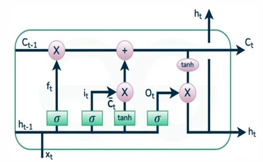
Each LSTM has four chain interacting communicative gates.
LSTM networks address the problem of vanishing gradients of RNN by splitting in three inner-cell gates and build memory cells to store information in a long range context [2]. As it has been seen from Figure 3, a typical LSTM cell is configured mainly by four gates: input gate, input modulation gate, forget gate and output gate. The input gate takes new input information from outside and process newly coming information. The Memory cell input gate takes input from the output of LSTM cell in the last iteration. Forget gate schedules when to forget the output data and thus selects the optimal time lag for the input sequence. Output gate takes all results and generate the output. The Cell and the hidden states are two states that are being transferred to the next cell.
The forget gate \(f_t\) deletes unimportant information from the previous time step and has an equation: \[f_t=\sigma(w_fh_{t-1}+u_fx_t+b_f) . \tag{8}\]
The input gate determines which information is significant through logistic and tanh activation functions. This gate has an equations:
\[\bar i_t=\sigma(w_ih_{t-1}+u_ix_t+b_i) , \tag{9}\]
\[\bar c_t=tanh(w_ch_{t-1}+u_cx_t+b_c), \tag{10}\]
\[i_t= \bar i_t*\bar c_t, \tag{11}\]
\[c_t= c_{t-1}*f_t+i_t. \tag{12}\]
The operation addition and multiplication are point operations. Finally in this unit the information to out put gate has an equation: \[o_t= \sigma(w_oh_{t-1}+u_ox_t+b_o), \tag{13}\] \[h_t= o_t*tanh(c_t), \tag{14}\] where \(w_f\),\(u_f\), \(w_i\), \(u_i\),\(w_c\), \(u_c\),\(w_o\),\(u_o\) are weights of the forget, input, input modulation and out put gets respectively. \(b\) the bias term. \(\sigma\) and \(tanh\) are the sigmoid(logistic) and hyperbolic tangent activation functions respectively and \(h_t\) is the hidden state.
CNN is a sub class of deep learning algorithms that exhibits spatial structures to extract relevant features from pattern of time series and serves for volatility prediction [34]. The structure of CNN has input layer which accepts the inputs, convolutional layers that are kernels of the CNN which works in convolution operation(Hadmard’s product), pooling layers which reduce the dimension by retaining the important imformation, fully connected layers(Dense) and flatten layers which changes into one dimension to the data and out put layers.
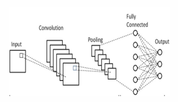
As it has been seen from Figure 4 at convolutional layer the input data operates the hadmard product with the kernel or filter and gives several results and these sent to ReLU activation function and mathematically these expressed as: \[f_i =g_i*t =\sum_{j=1}^{k}g_i[j]*t[i+j], \tag{15}\] where, \(f_i\) is the output of convolution operation at position \(i\), \(g_i\) the kernel convolutioned, \(g_i[j]\) is the \(j^{th}\) element of the kernel \(g_i\), \(k\) is the kernel size, \(t_i[i+j]\) is the \((i+j)^{th}\) element of the input \(t\) and \(*\) is element wise matrix multiplication(hadmard operation). The operation of ReLU(\(\sigma\)) activation function as: \[z_i =\sigma (f_i+b), \tag{16}\] where \(z_i\) is the out put and \(b\) is the bias term. The next process of the ReLU out put value goes to the maximum pooling or average pooling and finally changed to flatten data at fully connected layer.
The purpose of hybrid models is to improve the volatility prediction performance of the traditional GARCH family models. The features of volatility like clusters makes the inputs of deep learning models increase the prediction accuracy on result and estimated parameters [15,27,20,17,16,18]. As the result of this we design GARCH and CNN-LSTM, GARCH and LSTM, CNN and LSTM & GARCH and LSTM-CNN hybrid models. Therefore, GARCH-CNN-LSTM, GARCH-LSTM, CNN-LSTM and GARCH-LSTM-CNN hybrid models are utilized in the volatility prediction of S&P500 stock price.
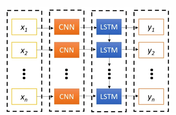
As shown in Figure 5 the conditional volatility result from GARCH (1,1) as a sequential data enters into convolutional layer and after convolutional operations passes to flatten layer and this out put as an input of the gets in LSTM.
In GARCH-LSTM-CNN model the conditional volatility obtained fron GARCH (1,1) serve as an input to the LSTM and out put of this sequencial data goes to the convolutional operations in CNN.
Since volatility is not directly observable (measurable quantity), we use the proxy for volatility in quantitatve way. To measure the forecasting performance of the designed model we consider the realized volatility interms of log return and the mathematical expression for log return and realized volatility respectively are:
\[R_t=ln\left(\frac{P_t}{P_{t-1}}\right), \tag{17}\] where \(P_t\) is the daily closed price of S&P 500 stock. \[\label{eq18} V=\sqrt{\frac{1}{T}\sum_{n=t}^{t+T-1}(R_t-\mu)^2}, \tag{18}\] where \(R_t\) is the log return at time \(t\) and \(\mu\) is the mean of the out sample return. Eq. (18) is the volatility interms of standard deviation of out sample( test data)in T rolling window. However, the most common proxy for daily variance forecasting and modeling the realized volatility is simply the daily squared returns \[V_d=\frac{1}{T}\sum_{i=1}^{T}R_i^2, \tag{19}\] where \(R_i\) is the return at time \(i\) in the day and \(T\) the number of daily return observations [1].
The performance of the model’s volatility forecasting is measured by comparing the forecasted volatility with the realized volatility in the out sample data using the metrics mean square error(MSE), root mean square error (RMSE) and the mean absolute error (MAE). MSE describes the average of the difference squares in the observed and predicted volatility. RMSE indicates the magnitude of the error in square root of the average square of the predicted and observed values, where as MAE shows the magnitude of absolute difference average of predicted and observed value. These equations are as follows:
Mean square error is: \[MSE= \frac{1}{n}\sum_{n=1}^{n}(\hat\sigma_t-\sigma_t)^2. \tag{20}\]
Root mean square error is: \[RMSE= \sqrt{\frac{1}{n}\sum_{n=1}^{n}(\hat\sigma_t-\sigma_t)^2}. \tag{21}\]
Mean absolute error is: \[MAE= \frac{1}{n}\sum_{n=1}^{n}\mid{\hat\sigma_t-\sigma_t\mid}, \tag{22}\] where \(\hat\sigma_t\) is the forecasted volatility , \(\sigma_t\) is the observed(actual) volatility value in time period \(t\) and n is number of out sample periods.
We took a historical trading days time series data of S&P500 stock closed price from 2019-06-07 to 2024-06-06 which has a total of 1259 samples. For simpler statistical analysis and stationarity this data is changed into log retuns. Furthermore, it splits into 2019-06-10 to 2023-03-08(944) for training, 2023-03-09 to 2023-10-30 (163) for validation and 2023-10-31 to 2024-06-06 (151) for test(out samples).
| Model | Error | AIC | SIC | Log | p-vale | p-value. |
| distribution | likelihood | \(\alpha\) | \(\beta\) | |||
| GARCH(1,1) | ND | -4.3414 | -4.3210 | 3990.59 | 0.0000 | 0.00000 |
| GARCH(1,1) | STD | -4.3741 | -4.3496 | 4012.23 | 0.0000 | 0.1020 |
| GARCH(1,1) | GED | -4.3684 | -4.3439 | 4008.56 | 0.0165 | 0.0250 |
| TGARCH(1,1) | ND | -4.3548 | -4.3302 | 4000.02 | 0.0012 | 0.0030 |
| TGARCG(1,1) | STD | -4.3909 | -4.3784 | 4017.55 | 0.0516 | 0.4270 |
| TGARCH(1,1) | GED | -4.3850 | -4.3564 | 4020.01 | 0.0064 | 0.2850 |
| EGARCH(1,1) | ND | -4.3570 | -4.3325 | 4001.39 | 0.0186 | 0.0251 |
| EGARCH(1,1) | STD | -4.4027 | -4.3741 | 4031.13 | 0.1951 | 0.6350 |
| EGARCH(1,1) | GED | -4.3865 | -4.3579 | 4020.97 | 0.0265 | 0.66 73 |
From Table 4, we observed that GARCH(1,1), TGARCH(1,1) and EGARCH(1,1) models under normal distribution(ND), student’s t-distribution(STD) and generalized error distribution(GED) assumptions of S&P 500 log return were selected as the candidate models using minimum Akaike information criteria(AIC), minimum Schwarz information criterion(SIC) and maximum log likelihood with significant p value of parameters( p-value less than 5%). Thus, based on the minimum information criteria, maximum log likelihood and significant coefficients, GARCH(1,1) with GED assumption for S&P500 log return is identified as the best performing model among the selected candidate models. The distribution is GED that reveals it is leptokurtic.
The conditional variance equation of S&P500 log return in GARCH(1,1)GED is: \[\label{eq3} \sigma^2_t=\alpha_0 + \alpha_1 \varepsilon^2_{t-1} +\beta_1\sigma^2_{t-1} , \tag{23}\] \[\label{e24} \sigma^2_t=0.0000036+0.1668\varepsilon^2_{t-1}+0.8145\sigma^2_{t-1} . \tag{24}\]
From Eq. (24) above indicates that the volatility of returns is persistent, with the sum of \(\alpha_1\) and \(\beta_1\) equal to 0.981(close to unity) which is mean reverting. Moreover, stationarity condition of \(\alpha_1+\beta_1< 1\) is satisfied and it shows that the conditional variance of S&P 500 return series is stable and predictable.
After the identification of GARCH(1,1), we estimated the conditional volatility of S&P 500 stock return and the forecasting performance is 0.0000286, 0.005352 and 0.004516 in mean squared error, root mean squared error and mean absolute error respectively in the out sample test data.
The fitness of the actual volatility which is the logarithmic return of S&P 500 with conditional volatility obtained from GARCH(1,1) in the training data and the test data with forecasted volatility are depicted in Figure 6.
We imported the units of CNN and LSTM from tensorflow and keras library in python software. From estimated conditional volatility keeping the size of training, validation and test data in GARCH(1,1), we trained this output conditional volatility into the input CNN -LSTM hybrid model with 20 timesteps(lookbacks),75% time splits, 11 number of folds and hyperparameters in 5. The selection of tunning or hyperparameter is trial and error(random search method) in minimum metrics.
| Model | Activation function | Pool size | kernel filters/units | Number of | Optimizer | epoch | Batch size |
| CNN | ReLU | 2 | 3 | 64 | Adam(lr=0.0001-0.0005) | 120-200 | 32 |
| LSTM | ReLU | 50 | Adam(lr=0.0001-0.0005) | 120-200 | 32 |
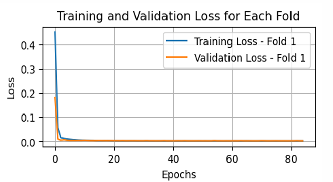
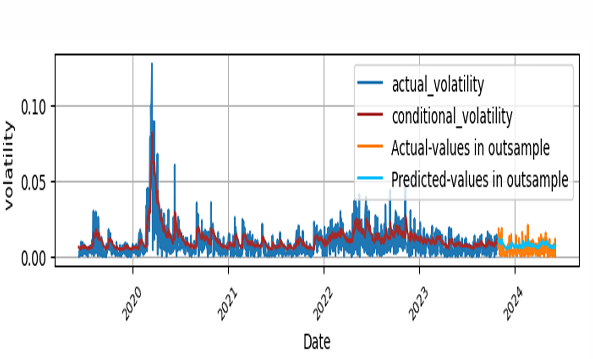
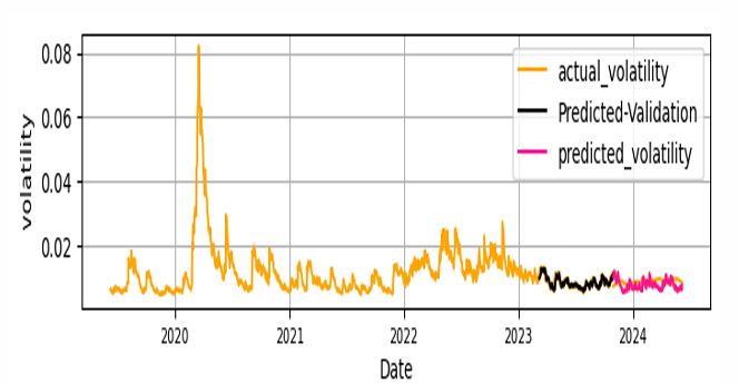
The loss value in the GARCH-CNN-LSTM training process is depicted in Figure 7 . Furthermore, the fitness of actual, predicted from GARCH and predicted volatility from GARCH-CNN-LSTM of out sample data set and the comparison of predicted and actual test data(realized volatility of the out samples set) is depicted in Figure 8.
The forecasting performance of GARCH-CNN-LSTM hybrid model in out sample data set by the loss functions MSE, RMSE and MAE is depicted in Table 6.
The experiment of GARCH-LSTM is processed by taking the output of GARCH(1,1) as the input for LSTM with the same training, validation and test set data size as GARCH-CNN-LSTM and the same kind and number of parameters and hyperparameters. The fitness of predicted versus test data is plotted at Figure 9.

Keeping the parameters and hyperparamers used for GARCH-LSTM and data S&P 500 stock return as the input for CNN integration into LSTM with the same size of training, validation and test data is carried out for CNN-LSTM hybrid model. Comparatively the performance of this model is stated at Table 6. Using the conditional volatility of GARCH(1,1) with the same size validation ,test data and hyper parametres as GARCH-CNN-LSTM only changng the order CNN and LSTM deep learning models the hybrid GARCH-LSTM-CNN is experimented and volatility forecasting performance in mean square error, root mean square error and mean absolute error is depicted at Table 6.
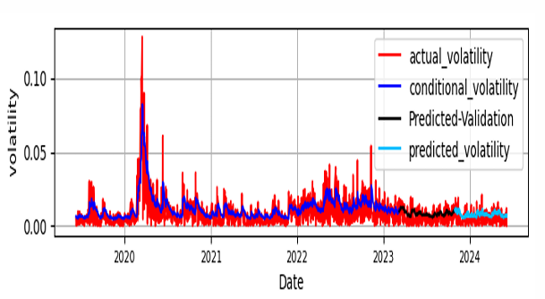
The loss value during the training process as well as the fitness of predictions with the actual data in training set, validation with actual data in validation set and with predictions in test data are depicted in Figure 10 and Figure 11 for CNN-LSTM and GARCH-LSTM-CNN models respectively.
From Table 6, the minimum values in mean square error, root mean square error and mean absolute errors we observe that GARCH-CNN-LSTM has the lowest values in the three metrics and GARCH-LSTM has the second lowest values, where as GARCH has the highest values which indicates that GARCH-CNN-LSTM is the most accurate model in forecasting the volatility of S&P 500 stock price and GARCH-LSTM is the second one. GARCH is the worest of all in the volatility predicting performance of the S&P 500 stock price. The S&P 500 stock price volatility prediction power of GARCH-LSTM-CNN less than GARCH-CNN-LSTM the sequential input and output matters.

| Metrics | GARCH | GARCH | GARCH | GARCH | |
| CNN-LSTM | LSTM | CNN-LSTM | LSTM-CNN | ||
| MSE | 0.00002865 | 0.00002524 | 0.00002741 | 0.00002813 | 0.000027631 |
| RMSE | 0.005352 | 0.005024 | 0.005235 | 0.005304 | 0.005256 |
| MAE | 0.004516 | 0.004218 | 0.004515 | 0.004685 | 0.004553 |
| GARCH | GARCH | GARCH | GARCH | ||
| CNN-LSTM | LSTM | CNN-LSTM | LSTM-CNN | ||
| GARCH | 0 | 0 | 0 | 0 | |
| GARCH-CNN-LSTM | 0 | 0 | 0 | 0 | |
| GARCH-LSTM | 0. | 0 | 0 | 0 | |
| CNN-LSTM | 0 | 0 | 0 | 0 | |
| GARCH-LSTM-CNN | 0 | 0 | 0 | 0 |
Table 7 shows the Diebold Mariano test results for the same number of outsample days ,the models have comparable accuracy as all the p-values are significant at 5% significant lablel. This indicates that each model has different volatility prediction performance in S&P 500 stock market dynamics.
Although deep learning algoriths have an ability of better forecasting in time series, they have drawbacks in parameter setting as tuning is based on trial and error depending on the nature of data [24].
Predicting future stock market trends is crucial for traders and investors seeking to mitigate risks. This study focuses on forecasting S&P 500 stock price volatility by combining econometric and deep learning models.
The volatility of S&P 500 stock return has been analyzed using symmetric GARCH, asymmetric TGARCH and EGARCH models, evaluated under normal, Student’s t and generalized error distributions. Based on the criteria in minimum Akaike Information Criterion (AIC) and maximum log-likelihood with significant statistical coefficients, the GARCH(1,1) model with a generalized error distribution outperforms other GARCH extensions in predicting S&P 500 stock price volatility. Additionally, we computed the conditional volatility of S&P 500 stock prices during the study period, providing input for hybrid CNN and LSTM neural network models.
The integration of GARCH with LSTM in forecasting S&P 500 stock price volatility performs effectively, evidenced by low MSE, RMSE, and MAE values in out-of-sample data. GARCH captures spatial volatility features such as volatility clustering, while LSTM captures long-term memory persistence. Similarly, the hybrid model GARCH-CNN-LSTM slightly outperforms in volatility forecasting, leveraging CNN’s ability to recognize spatial patterns in the time series data, as indicated by the same metrics and out-of-sample data. The combination of CNN and LSTM shows the lowest performance in terms of high MSE, RMSE, and MAE values on the same out-of-sample data. When forecasting the volatility of S&P 500 stock prices, the GARCH-LSTM-CNN hybrid model performs better than CNN-LSTM but not as well as either GARCH-LSTM or GARCH-CNN-LSTM hybrid models.
In this article, we focus only on the closing price of the stock. However, incorporating additional factors such as volume, trading activity, and optimizing parameters and hyperparameters selection methods will enhance the accuracy of predicting S&P 500 stock price volatility.
In summary GARCH-CNN-LSTM is best out performs in the forecasting volatility of S&P 500 stock price upto 13% accuracy improvement in the study period and GARCH-LSTM is the second most out performs well. Improved predictive abilities of forecasting the volatility of S&p 500 stock price is pivotal for the decision of finance and risk management in stock market trading.
The authors have no competing interests to declare that are relevant to the content of this article.
No funding was received for conducting this study
The data presented in this study is accessible upon request from the corresponding author.