
A fundamental assumption in the field of international business is that the performance outcomes of multinational enterprises (MNEs) differ from those of purely domestic firms. Portfolio diversification can be used to explain how global diversification of MNE activities affects cross-border risk and performance. Portfolio diversification theory suggests that by offsetting idiosyncratic volatility caused by exogenous events (e.g., exchange rate fluctuations) and by operating passively through geographically underperforming assets, MNEs can reduce the total variance and covariance of their portfolios, resulting in a well-diversified portfolio [10,23,3,17].
Portfolio theory emphasizes the risk-reducing benefits of investing in a set of assets whose returns are not perfectly correlated [1,18]. In the context of international business activities, the application of portfolio theory suggests that greater geographic scope provides risk diversification opportunities that can reduce overall portfolio variance and improve risk-return performance outcomes, especially in geographic markets with imperfectly correlated market characteristics [15,20,22]. When there is imperfect correlation between different regions, the activities of multinational firms in different countries may exhibit lower risk than the sector-weighted average of those operating independently in each regional market [13,9,5]. This risk diversification effect can even be realized through passive management, where diversification reduces the variance of portfolio returns as long as lower covariances exist in selected geographic markets [21,16,11]. Since portfolio diversification activities can involve significant implementation costs, passive management of portfolio assets is often considered superior to more active and expensive portfolio management.
The optimization of investment portfolios has long been a central concern in the investment management industry and continues to be a subject of research. [7] examined stock market investments and employed the fund standardization method to represent portfolio returns and calculate portfolio risk. By integrating this approach with a genetic algorithm, the study identified the optimal portfolio, demonstrating that this method could effectively achieve stable returns while minimizing risk. The findings suggested that the standardized fluctuation of investment funds accurately reflected the relative relationship between stocks.
[9] clarified that portfolio optimization involves identifying the efficient frontier between representative returns and risks. The study proposed the use of the Swarm Intelligence (SI) method to address computational challenges associated with portfolio optimization. Meanwhile, [6] introduced predictive modeling into stock market portfolio optimization by developing a machine learning algorithm for stock return prediction and combining it with a mean-at-risk model for portfolio selection. The hybrid approach significantly enhanced investment returns.
Furthermore, [4] explored the role of performance-based regularization (PBR) and cross-validation in portfolio optimization. Experimental analysis demonstrated that the PBR model functioned as a robust optimization framework by incorporating new uncertainties in mean-variance and mean-conditional-value-at-risk (mean-CVaR) problems. Additionally, the k-fold cross-validation algorithm proved effective in calibrating the right-hand side of PBR constraints.
[12] developed a robust optimal solution model for portfolio optimization based on real data and traced the robust linear programming model back to the standard form of linear programming. Both real and simulated data indicated that this approach improved portfolio stability and reduced risk. Lastly, [2] introduced the concept of Entropy Value-at-Risk (EVaR), demonstrating that it was strictly monotonic across a broad range of sub-value domains, including all continuous distributions. Compared to Value-at-Risk (VaR) and Conditional Value-at-Risk (CVaR), EVaR allowed the portfolio rate to be linearly dependent on decision variables, leading to optimal allocation strategies in large-scale portfolio samples.
This paper analyzes the basic elements involved in linear programming problems and establishes the standard form of linear programming applicable to investment decisions. Pointing out the deficiencies of the traditional portfolio theory centered on the mean-variance model and the expected utility theory, combined with the fuzzy decision-making theory, it proposes a stochastic fuzzy portfolio model that takes into account the risk characteristics of investors. Considering the different psychological characteristics of investors facing the stochasticity of the securities market and the different psychological needs of investors, the return of assets is regarded as a stochastic fuzzy variable, and the stochastic fuzzy objective affiliation function of the portfolio is established, and the steps of model solving are given. Discuss the portfolio return strategies under different risk preference characteristics or different emotional states of investors. Empirical optimization of fund portfolio strategies is carried out in conjunction with sample firms.
Production and business management often put forward how to rationalize the arrangement, so that human and material resources and other resources are fully utilized to obtain the maximum benefit, which is called the planning problem. Usually called the real world people care about, the actual object of research for the prototype. The mathematical model of the planning problem contains three components:
(1) Decision variables, refers to the decision makers to achieve the planning objectives to take programs, measures, is the problem to determine the unknown quantity.
(2) Objective function, refers to the purpose of the problem to achieve the requirements, expressed as a function of the decision variables.
(3) Constraints, refers to the decision variable to take the value of the limitations of the various available resources, expressed as an equation or inequality containing the decision variable.
If in the mathematical model of the planning problem, the decision variable is a controllable continuous variable. The objective function and constraints are linear, such models are called mathematical models of linear programming problems.
The standard form of linear programming is given below as: \[\label{GrindEQ__1_} \begin{cases}\min \quad c_{1} x_{1} +c_{2} x_{2} +\cdots +c_{n} x_{n} ,\\ \begin{array}{cc} \text{s.t.} & {\left\{\begin{array}{c} {a_{11} x_{1} +a_{12} x_{2} +\cdots +a_{1n} x_{n} =b_{1} }, \\ {a_{21} x_{1} +a_{22} x_{2} +\cdots +a_{2n} x_{n} =b_{2} }, \\ {\vdots } \\ {a_{m1} x_{1} +a_{m2} x_{2} +\cdots +a_{mn} x_{n} =b_{m} }, \end{array}\right. } \\ {} & {x_{1} ,x_{2} ,\cdots x_{n} \ge 0}. \end{array} \end{cases} \tag{1}\]
Write in compact format: \[\label{GrindEQ__3_} \begin{cases}{\min } {\sum\limits_{j=1}^{n}c_{j} x_{j} },\\ \begin{array}{cc} \text{s.t.} & {\sum\limits_{j=1}^{n}a_{ij} x_{j} =b_{j} i=1,2,\cdots m}, \;\;\; {x_{j} \ge 0,\;\;\;j=1,2,\cdots n,} \end{array} \end{cases} \tag{2}\] and matrix forms: \[\begin{cases} \label{GrindEQ__5_} {\min } {c^{T} x}, \\ \text{s.t.} {Ax=b}, \;\; {x\ge 0} .\end{cases} \tag{3}\]
Among them: \[\label{GrindEQ__6_} c=\left[\begin{array}{c} {c_{1} } \\ {c_{2} } \\ {\vdots } \\ {c_{n} } \end{array}\right],A=\left[\begin{array}{cccc} {a_{11} } & {a_{12} } & {\cdots } & {a_{1n} } \\ {a_{21} } & {a_{22} } & {\cdots } & {a_{2n} } \\ {\vdots } & {\vdots } & {\ddots } & {\vdots } \\ {a_{m1} } & {a_{m2} } & {\cdots } & {a_{mn} } \end{array}\right],x=\left[\begin{array}{c} {x_{1} } \\ {x_{2} } \\ {\vdots } \\ {x_{n} } \end{array}\right],b=\left[\begin{array}{c} {b_{1} } \\ {b_{2} } \\ {\vdots } \\ {b_{n} } \end{array}\right] . \tag{4}\]
For general linear programming problems, it is possible for the objective function to be extremely small or extremely large, and there may be inequality constraints in addition to equation constraints. There may not be a non-negative constraint for every variable \(x_{j}\). For a general linear programming problem, first reduce it to standard form.
1) If the objective is to find the maximum value \(\max c^{T} x\) is equivalent to \(\min -c^{T} x\).
2) If the constraints are inequality constraints: \[\label{GrindEQ__7_} \sum\limits_{j=1}^{n}a_{ij} x_{j} =b_{j} . \tag{5}\]
Equivalent: \[\label{GrindEQ__8_} \left.\begin{array}{l} {\sum\limits_{j=1}^{n}a_{ij} x_{j} +x_{n+i} =b_{i} },\;\;\;{x_{n+i} \ge 0}. \end{array}\right. \tag{6}\]
At this point \(x_{n+i}\) is said to be the slack variable. Inequality constraints: \[\label{GrindEQ__9_} \sum\limits_{j=1}^{n}a_{ij} x_{j} \ge b_{j} . \tag{7}\]
Equivalent: \[\label{GrindEQ__10_} \left.\begin{array}{l} {\sum\limits_{j=1}^{n}a_{ij} x_{j} -x_{n+i} =b_{i} }, \;\;\;\; {x_{n+i} \ge 0}. \end{array}\right. \tag{8}\]
At this point \(x_{n+i}\) is said to be the residual variable.
For linear programming problems, there are mainly the following solution methods:
1) Graphical solution, which has the advantage of being intuitive. The disadvantage is that it is only applicable to the case of two variables. The specific steps are to establish a coordinate system and represent the constraints on a graph. Establish the range of solutions that satisfy the constraints plot the graph of the objective function to determine the optimal solution.
2) Simplex form method, whose method steps are more complex, including the artificial variable method, two-stage method, etc., and some people propose to improve the method. As this paper in the linear programming problem solving with the help of Matlab programming, so the process of the above solution will not be repeated.
Combined with the fuzzy theory, the fuzzy decision theory is established in solving the research of multi-objective decision-making problems [24,14]. This fuzzy decision-making model includes two elements: fuzzy objectives and fuzzy constraints. Let the set of real numbers \(R,X\) be the cluster of fuzzy sets defined on it, \(G\) be the fuzzy objective on the fuzzy set, \(C\) be the fuzzy constraint, and the fuzzy decision is \(D=G\cap C\), i.e., the affiliation function of \(D\) is: \[\label{GrindEQ__11_} \mu _{D} (x)=\min (\mu _{G} (x),\mu _{C} (x))\quad \forall x\in X . \tag{9}\]
Similarly, if there are \(m,n\) fuzzy objective, fuzzy constraint respectively, the fuzzy decision is defined as follows: \[\label{GrindEQ__12_} D=\left\{\begin{array}{c} {G_{1} \cap G_{2} \cap \cdots \cap G_{m} } \end{array}\right\}\cap \left\{\begin{array}{c} {C_{1} \cap C_{2} \cap \cdots \cap C_{n} } \end{array}\right\} . \tag{10}\]
Then its fuzzy affiliation function is: \[\label{GrindEQ__13_} \mu _{D} (x)=\min \left\{\mu _{G_{1} } (x),\mu _{G_{2} } (x),\cdots ,\mu _{G_{n} } (x),\mu _{C_{1} } (x),\mu _{C_{2} } (x),\cdots ,\mu _{C_{n} } (x)\right\} . \tag{11}\]
From the above definitions, it can be seen that fuzzy objectives are no different from fuzzy constraints in a fuzzy environment.
The maximization decision criterion for non-fuzzy numbers is proposed: \[\label{GrindEQ__14_} D^{*} =\left\{x^{*} \in X|x^{*} =\arg \max (\mu _{D} (x))\right\}=\arg \max \{ \min (\mu _{G} (x),\mu _{C} (x))\} . \tag{12}\]
If given \(m\) fuzzy objective and \(n\) fuzzy constraints: \[\begin{aligned} \label{GrindEQ__15_} {D{}^{*} } {=} & {\left\{x^{*} \in X|x^{*} =\arg \max (\mu _{D} (x))\right\}} \notag\\ {} {=} & {\arg \max \left\{\min (\mathop{\scriptscriptstyle\leftharpoondown}\limits^{\displaystyle\rightharpoonup} \mu _{G_{1} } (x),\mathop{\scriptscriptstyle\leftharpoondown}\limits^{\displaystyle\rightharpoonup} \mu _{G_{2} } (x),\cdots ,\mu _{G_{m} } (x),\mu _{C_{1} } (x),\mathop{\scriptscriptstyle\leftharpoondown}\limits^{\displaystyle\rightharpoonup} \mu _{C_{2} } (x),\cdots ,\mu _{C_{m} } (x))\right\}.} \end{aligned} \tag{13}\]
Based on the proposed fuzzy decision theory, the first fuzzy decision-based portfolio model is developed and applied to the portfolio problem of bonds. The idea of the study is as follows, assuming that the portfolio contains \(n\) security and the market has a total of \(m\) possible states. The range of investor’s target return in the \(k\)rd market state is \([R_{k}^{{\rm min}} ,R_{k}^{{\rm max}} ]\). For the \(i\)th security, the upper and lower bounds of investor’s investment ratio are \([x_{i}^{{\rm min}} ,x_{i}^{{\rm max}} ]\). Let \(R_{ik}\) denote the return of the \(i\)th security in the \(k\)th market, then \(R_{k} (x)=\sum R_{ik} x_{i}\) is the expected return of the portfolio in the \(k\)th market. The investor’s satisfaction with the investment return can be represented by a linear affiliation function with the following segments: \[\label{GrindEQ__16_} \mu _{k} (R_{k} (x))=\left\{\begin{array}{ll} {0} & {\quad \text{if}\quad R_{k} (x)<R_{k}^{min} }, \\ {\frac{R_{k} (x)-R_{k}^{min} }{R_{k}^{max} -R_{k}^{min} } } & {\quad \text{if}\quad R_{k}^{min} \le R_{k} (x)\le R_{k}^{max} }, \\ {1} & {\quad \text{if}\quad R_{k} (x)\ge R_{k}^{max} }. \end{array}\right. \tag{14}\]
The portfolio is then modeled as follows: \[\label{GrindEQ__17_} \begin{cases} {\max } & {\lambda }, \\ \text{s.t.} & {\mu _{k} (R_{k} (x))\ge \lambda }, \;\; {\sum\limits_{i=1}^{n}x_{i} =1} ,\;\; {x_{i}^{\min } \le x_{i} \le x_{i}^{\max } }. \end{cases} \tag{15}\]
Traditional financial theory assumes that investors are psychologically endowed with the qualities of rational expectations, risk aversion and utility maximization. On this basis, the mean-variance theory and the strictly axiomatic expected utility theory have been developed as modeled descriptions of people’s rational behavior when making decisions under uncertainty. A series of strict axiomatic assumptions of expected utility theory have been seriously challenged by relevant psychological experiments, and phenomena such as the certainty effect, the same-ratio effect, the isolation effect, the firing effect, preference reversal, and probabilistic insurance have shown that people’s actual decision-making behaviors deviate from expected utility theory. At the same time, financial scientists have found a large number of market anomalies in their research that cannot be explained by traditional financial theories.
For a long time, the traditional portfolio theory centered on mean-variance model and expected utility theory has at least the following limitations.
(1) Rational man assumption: traditional financial theory treats investors’ decision-making behavior as a black box, ignoring the impact of investors’ emotions, time pressure and other factors on decision-making.
(2) Consistency of investor risk attitudes assumption: psychological experiments have shown that investors are not homogeneous and have different risk preferences and behavioral styles. Investors are not always risk averse, and sometimes pursue risk, both conservative and adventurous psychological characteristics. Investors are actually loss averse rather than risk averse [8].
(3) Efficient Market Hypothesis: The Efficient Market Hypothesis (EMH) is a central proposition of modern mainstream financial theory and even mainstream economics. One of its basic inferences is that changes in asset prices or returns follow a “random walk” process, it is impossible to expect future changes in asset prices and returns. The basic idea behind the test of whether a market is efficient is to compare actual returns with expected returns. If they do not, the market is considered inefficient.
Subjective expected utility theory (SEU) introduces the subjective utility of human beings, although it is closer to reality than expected utility theory (EU). However, both assume that investors are completely rational, which is obviously contrary to the actual situation.
In the actual decision-making process, investors are often affected by their own psychological state, emotions and external environment, showing limited rationality, decision-making bias. That is, the actual decision-making behavior is often inconsistent with the strategy given by EU or SEU theory. In view of the above shortcomings of the expected utility theory, the non-expected utility theory is proposed by analyzing and summarizing the actual data. In order to solve the problem of decision-making under uncertain conditions, and on this basis, behavioral economics has been gradually developed, and the corresponding behavioral finance theory effectively explains the above market anomalies through the introduction of the analysis of investor behavior and psychology.
In this paper, considering that investors face the double uncertainty factors of stochastic and fuzzy in the securities market, the return of assets is regarded as a stochastic fuzzy variable. And considering the psychological needs of investors with different risk characteristics, it establishes stochastic fuzzy variables considering investors’ risk characteristics. Further, the fuzzy expected return affiliation function is established on the basis of prospect theory. And use the weighted very large-very small operator to consider the difference of investment objectives of different investors, and construct the stochastic fuzzy portfolio model considering investors’ risk characteristics.
On the basis of plausibility theory, it is assumed that the security return \(\bar{F}\) is a random fuzzy variable and \(\bar{\tilde{r}}_{i}\) obeys a normal random distribution with mean L-R fuzzy variable, i.e. \(\bar{\tilde{r}}_{i} \sim N(\tilde{M}_{i} ,\sigma _{i}^{2} ),i=1,2,…,n\), whose mathematical expression is: \[\label{GrindEQ__18_} \left\{\begin{array}{l} {f_{i} (z)=\frac{1}{\sqrt{2\pi } \sigma _{i} } \exp \left[-\frac{(z-\tilde{M}_{i} )^{2} }{2\sigma _{i}^{2} } \right]}, \\ {\mu _{\tilde{M}_{i} } (s_{i} )=\left\{\begin{array}{c} {L\left(\frac{m_{i} -s_{i} }{\alpha _{i} } \right),m_{i} -\alpha _{i} \le s_{i} \le m_{i} }, \\ {R\left(\frac{s_{i} -m_{i} }{\beta _{i} } \right),m_{i} \le s_{i} \le m_{i} +\beta _{i} } ,\end{array}\right. } \end{array}\right. \tag{16}\] where \(L(\cdot )\) and \(R(\cdot )\) are nonincreasing, upper semicontinuous functions and \(L(0)=R(0)=1,L(1)=R(1)=0\). Parameters \(\alpha _{i}\) and \(\beta _{i}\) denote the parameters to the left and right of the fuzzy number of the mean of the \(i\)th security, respectively, and \(\alpha _{i}\) and \(\beta _{i}\) are both positive, and \(n\) represents the type of security.
Risk-seeking investors focus on investment returns, leading to overestimation of the affiliation function of the security’s return. Risk-averse investors focus on investment risk, resulting in an underestimation of the affiliation function of the security return. According to the concavity of the fuzzy variable affiliation function, the fuzzy yield affiliation function \(u_{\tilde{\hbar }} (s_{i} ),i=1,2,…,n\) is proposed to take into account the risk characteristics of investors, and its mathematical expression is: \[\label{GrindEQ__19_} u_{i} \left(s_{i} \right)=\left\{\begin{array}{c} {1-\left(\frac{m_{i} -s_{i} }{\alpha _{i} } \right)^{k} ,m_{i} -\alpha _{i} \le s_{i} \le m_{i} }, \\ {1-\left(\frac{s_{i} -m_{i} }{\beta _{i} } \right)^{k} ,m_{i} \le s_{i} \le m_{i} +\beta _{i} }, \end{array}\right. \tag{17}\] where \(u_{i} (s_{i} )\) is a convex function when \(k>1\), denoting a risk-seeking investor. When \(k=1\) when \(u_{i} (s_{i} )\) is a linear function, denoting a risk-averse investor. When \(k<1\) when \(u_{i} (s_{i} )\) is a concave function, indicating risk-neutral investors.
Substituting Eq. (17) into equation (16), the stochastic fuzzy rate of return \(i=1,2,\ldots n\) can be obtained by considering the risk characteristics of the investment information, and its mathematical expression is: \[\label{GrindEQ__20_} \begin{cases} {f_{i} (z)=\frac{1}{\sqrt{2\pi } \sigma _{i} } \exp \left[\cdots \frac{(z-\tilde{M}_{i} )^{2} }{2\sigma _{i}^{2} } \right]}, \\ {\mu (s_{i} )=\left\{\begin{array}{c} {L^{N} \left(\frac{m_{i} -s_{i} }{\alpha _{i} } \right)=1-\left(\frac{m_{i} -s_{i} }{\alpha _{i} } \right)^{k} ,m_{i} -\alpha _{i} \le s_{i} \le m_{i} }, \\ {R^{N} \left(\frac{s_{i} -m_{i} }{\beta _{i} } \right)=1-\left(\frac{s_{i} -m_{i} }{\beta _{i} } \right)^{k} ,m_{i} \le s_{i} \le m_{i} +\beta _{i} }. \end{array}\right. } \end{cases} \tag{18}\]
Thus, the affiliation function of the stochastic fuzzy collection rate \(\bar{r}_{i}^{kv}\) considering the investment if risk characteristics is: \[\label{GrindEQ__21_} \mu_i^k(\upsilon) = \sup \left\{ \mu_i^k(s) \mid \upsilon_i \sim N(s_i, \sigma_i^2) \right\}, \quad \upsilon_j \in \Gamma, \quad i = 1,2, \dots, n. \tag{19}\]
In this case, is the ensemble of positive-thought random fractions, and \(\mu _{i}^{R^{{'} } } (\upsilon _{i} )\) is the degree to which the random fuzzy yield \(\bar{r}_{i}^{kv}\) is equal to \(\bar{\upsilon }\).
Let \(\bar{r}_{i}^{xc}\) represents the random fuzzy return of security \(i\), then \(\bar{\tilde{f}}=\sum\limits_{i=1}^{n}\bar{\bar{r}}_{i}^{RC} x_{i}\) represents the random fuzzy return of the portfolio. According to the definition (22) that \(\bar{\tilde{f}}\) is a random fuzzy variable, the portfolio return \(\bar{\tilde{f}}\) affiliation function: \[\begin{aligned} \label{GrindEQ__22_} \mu_j(\bar{u}) =& \sup_{\tau} \left\{ \min_{1 \leq k \leq n} \mu_{\tau_j}^{RC} (\bar{u}_i) \Bigg| \bar{u} = \sum\limits_{i=1}^{n} \bar{U}_i x_i \right\} \notag\\ =& \sup_{s} \left\{ \min_{1 \leq k \leq n} \mu_{\tau_j}^{RC} (s_i) \Bigg| \bar{u} \sim N \left( \sum\limits_{i=1}^{n} s_i x_i, \sum\limits_{i=1}^{n} \sum\limits_{j=1}^{n} \sigma_{j} x_i x_j \right) \right\}. \end{aligned} \tag{20}\]
Among them: \[\begin{aligned} \label{GrindEQ__23_} \bar{u} \in Y, Y =& \left\{ \sum\limits_{i=1}^{n} \bar{U}_i x_i \Bigg| \bar{U}_i \in \Gamma, j = 1,2, \dots, n \right\}, \notag\\ \bar{U} =& (\upsilon_1, \upsilon_2, \dots, \upsilon_n),\notag \\ s =& (s_1, s_2, \dots, s_n) , \end{aligned} \tag{21}\] where \(\sigma _{ij}\) denotes the covariance of security \(i\) and security \(j\).
Combine SP/A theory and prospect theory to propose a behavioral portfolio model, and use the target probability to measure the uncertainty level of the portfolio to reach the goal. Investors in the financial market have multiple investment objectives, which not only require the maximization of returns. It also requires that the target probability \(\tilde{P}=\Pr \left\{\omega |\sum\limits_{i=1}^{n}\bar{r}_{i}^{RC} x_{i} \ge f\right\}\) be maximized for a certain level \(f\) of return. Substituting Eq. (21) into \(\tilde{P}\) yields the affiliation function of the target probability \(\tilde{P}\) of the portfolio: \[\label{GrindEQ__24_} \begin{array}{rcl} {\mu _{\tilde{P}} (p)} & {=} & {{\mathop{\sup }\limits_{\bar{u}}} \left\{\mu _{\bar{f}} (\bar{u})|p=\Pr \left\{\omega |\bar{u}(\omega )\ge f\right\}\right\}} \\ {} & {=} & {{\mathop{\sup }\limits_{s}} \min _{1\le i\le n} \left\{\begin{array}{cc} {\mu _{\tilde{u}_{i} }^{RC} (s_{i} )|} & {\begin{array}{c} {\Pr \left\{\omega |\bar{u}(\omega )\ge f\right\}} \\ {\bar{u}\sim N\left(\sum\limits_{i=1}^{n}s_{i} x_{i} ,\sum\limits_{i=1}^{n}\sum\limits_{j=1}^{n}\sigma _{ij} x_{i} x_{j} \right)} \end{array}} \end{array}\right\}}. \end{array} \tag{22}\]
Since \(\tilde{P}=Pr\left\{\omega |\sum\limits_{i=1}^{n}\bar{r}_{i}^{nc} x_{i} \ge f\right\}\) is a random fuzzy variable, solving for the maximum value of probability \(\tilde{P}\) is a fuzzy bounded problem. Use possibility planning to determine the extent to which probability \(\tilde{P}\) satisfies the investor’s fuzzy objective \(\tilde{G}_{p}\): \[\label{GrindEQ__25_} \prod _{\tilde{p}}(\tilde{G}_{p} ) ={\mathop{\sup }\limits_{p}} \min \left\{\mu _{\tilde{p}} (p),\mu _{\tilde{G}_{p} } (p)\right\} , \tag{23}\] where the investor’s expected return \(f\) is the interval fuzzy number. The degree to which the expected return satisfies the investor needs to be considered on the basis of Eq. (23) in order to turn the portfolio model into a well-bounded problem.
When making multi-objective investment decisions, investors with different risk characteristics have different preferences for the objective function. In order to be able to meet the needs of investors’ psychological characteristics, the weighted great-extremely small operator is introduced into the model, and the minimum value of the degree of affiliation in the weighted expected return and the target probability is used to indicate the degree to which a certain portfolio meets the psychological expectations of investors, i.e.: \[\label{GrindEQ__26_} U(x)=\min \left\{\frac{1}{\lambda _{1} } \prod _{\tilde{p}}(\tilde{G}_{p} ) ,\frac{1}{\lambda _{2} } \mu _{\tilde{G}_{f} } (f)\right\} , \tag{24}\] where \(\lambda _{1} +\lambda _{2} =1,\lambda _{1} >0,\lambda _{2} >0,\lambda _{1}\) and \(\lambda _{2}\) denote the investor’s target weights for the target probability and expected return, respectively.
The investor’s objective is to find a portfolio that makes it possible to maximize the satisfaction of his or her psychological expectations. According to Eq. (25), the stochastic fuzzy portfolio model that takes into account the risk characteristics of the investor under the condition that short selling is not allowed is: \[\label{GrindEQ__27_} \begin{cases}\max \min \left\{ \frac{1}{\lambda_1} \prod_{P} (\tilde{G}_p), \frac{1}{\lambda_2} \mu_{G_r}(\mathcal{F}) \right\}, \\ \text{s.t. } \lambda_1 + \lambda_2 = 1, \;\; \lambda_1 > 0, \quad \lambda_2 > 0, \;\;\sum\limits_{i=1}^{n} x_i = 1, \;\;0 \leq x_i \leq u_i, \quad i = 1,2, \dots, n, \end{cases} \tag{25}\] where \(u_{i}\) denotes the maximum investment weight of the \(i\)nd security.
Step 1: Generate the investor’s fuzzy expected return and target probability affiliation function according to Eq. (23) and Eq. (24), respectively.
Step 2: Set \(q\leftarrow \min \left(\frac{1}{\lambda } ,\frac{1}{\lambda } \right)\) and solve the model for the optimal solution \(x(q)\) and the optimal value \(Z(q)\). If \(Z(q)\ge g_{F}^{-1} (\lambda _{2} q)\), the operation is stopped. In this case, \(x(q)\) is the optimal weight of the model. Otherwise, proceed to the next step.
Step 3: Set \(q\leftarrow 0\) and solve the model for the optimal solution \(x(q)\) and optimal value \(Z(q)\). If \(Z(q)\le g_{F}^{-1} (\lambda _{2} q)\), stop the computation. In this case, \(x(q)\) the degree of satisfying the investor’s psychological expectations is 0. The fuzzy parameters of expected return and target probability should be reset or the investment in the security for the period should be abandoned. Otherwise, proceed to the next step.
Step 4: Intersection of \(Z(q)\) and \(g_{F}^{-1} (\lambda _{2} q)\) exists. Set \(R_{q} \leftarrow \min \left(\frac{1}{\lambda } ,\frac{1}{\lambda _{r} } \right)\) and \(L_{q} \leftarrow 0\).
Step 5: Set \(q\leftarrow \frac{R_{q} +L_{q} }{2}\).
Step 6: Calculate the optimal solution \(x(q)\) and the optimal value \(Z(q)\) of the model. If \(Z(q)=g_{F}^{-1} (\lambda _{2} q)^{1}\), stop the operation and \((x(q),q)\) is equal to \((x^{*} ,h^{*} )\). If \(Z(q)<g_{F}^{-1} (\lambda _{2} q)\), set \(R_{q} \leftarrow q\) and return to step 5. If \(Z(q)>g_{F}^{-1} (\lambda _{2} q)\), set \(L_{q} \leftarrow q\) and return to step 5.
In order to prove the validity and feasibility of the above model, this study takes 5 stocks in Shanghai Stock Exchange as the research data, and the trapezoidal possibility distribution of their investment returns is shown in Table 1.
| Assets | Trapezoidal fuzzy number |
| Asset 1 | ( 0.056,0.023,0.054,0.097 ) |
| Asset 2 | ( 0.095,0.116,0.077,0.143 ) |
| Asset 3 | ( 0.118,0.138,0.096,0.125 ) |
| Asset 4 | ( 0.134,0.168,0.113,0.165 ) |
| Asset 5 | ( 0.128,0.213,0.157,0.223 ) |
Based on the historical data, expert experience, market forecast analysis and other information, combined with the gradient fuzzy number calculation method, the trapezoidal possibility distribution of the investment return rate of five risky assets is obtained.
This subsection focuses on how investor risk preferences affect investment portfolios when one of the investors’ subjective psychological factors, optimistic pessimism, is certain. Taking the neutrosophic mood state as an example, the model is solved separately to obtain the portfolio results of investors with different risk preferences.
The portfolio of risk-averse investors is shown in Table 2. As can be seen from the table, for risk-averse investors, their investment risk and return are 7.87% and 15.32% respectively when their portfolio realizes the optimal investment ratio.
| Risk (%) | 7.52 | 7.53 | 7.54 | 7.85 | 7.86 | 7.87 |
| Earnings(%) | 12.33 | 12.63 | 13.06 | 13.51 | 14.22 | 15.32 |
| \(x_1 \) | 0.4000 | 0.4000 | 0.2864 | 0.2399 | 0.1824 | 0.1000 |
| \(x_2 \) | 0.4000 | 0.2536 | 0.1856 | 0.1968 | 0.1404 | 0.1000 |
| \(x_3 \) | 0.2000 | 0.2000 | 0.1000 | 0.2000 | 0.2000 | 0.4000 |
| \(x_4 \) | 0.2000 | 0.2000 | 0.2000 | 0.3000 | 0.3000 | 0.3000 |
| \(x_5 \) | 0.3000 | 0.2367 | 0.3005 | 0.4123 | 0.4532 | 0.5000 |
The risk-neutral investor’s portfolio is shown in Table 3, with a maximum risk and return on investment of 8.97% and 14.33%.
| Risk (%) | 8.89 | 8.91 | 8.92 | 8.95 | 8.96 | 8.97 |
| Earnings(%) | 12.34 | 13.15 | 13.46 | 13.98 | 14.05 | 14.33 |
| \(x_1 \) | 0.5000 | 0.3000 | 0.231 | 0.2136 | 0.2104 | 0.1529 |
| \(x_2 \) | 0.4000 | 0.2235 | 0.1245 | 0.2131 | 0.2133 | 0.2000 |
| \(x_3 \) | 0.3000 | 0.1200 | 0.3000 | 0.2000 | 0.1500 | 0.3000 |
| \(x_4 \) | 0.2000 | 0.2000 | 0.2000 | 0.3051 | 0.2000 | 0.4000 |
| \(x_5 \) | 0.1000 | 0.3621 | 0.3458 | 0.4030 | 0.3000 | 0.5000 |
The risk-seeking investor’s portfolio is shown in Table 4 and the maximum risk and return on investment is 11.23% and 15.67%.
| Risk (%) | 11.04 | 11.05 | 11.06 | 11.21 | 11.22 | 11.23 |
| Earnings(%) | 13.47 | 13.62 | 13.89 | 14.36 | 14.78 | 15.67 |
| \(x_1 \) | 0.3000 | 0.3000 | 0.2683 | 0.2352 | 0.2193 | 0.2000 |
| \(x_2 \) | 0.4000 | 0.2342 | 0.2100 | 0.1563 | 0.2011 | 0.3000 |
| \(x_3 \) | 0.2000 | 0.2000 | 0.1253 | 0.2000 | 0.2000 | 0.1000 |
| \(x_4 \) | 0.1000 | 0.2000 | 0.2100 | 0.2300 | 0.3000 | 0.1000 |
| \(x_5 \) | 0.2000 | 0.3204 | 0.3244 | 0.4253 | 0.2634 | 0.4000 |
In summary, when investor sentiment is certain, the trend of investment ratios of investors with risk-averse, risk-neutral, and risk-seeking risk preferences is consistent. All of them realize the optimal investment ratio by reducing the ratio of lower-yielding asset 1 and asset 2 and increasing the ratio of high-yielding asset 5. The more one invests in low-yielding assets, the lower the investment risk. Similarly, the more you invest in high-yield assets, the higher the investment risk.
For investors with different risk preferences, it does not matter whether the return on assets is a triangular fuzzy number or a trapezoidal fuzzy number. Its portfolio return and risk are inversely proportional to the sensitivity of risk, the more sensitive the investor is to risk, i.e., the more risk-averse the risk preference. The lower their portfolio return and risk, again proving the impact of investors’ subjective psychological factors on investment decisions.
Similar to the previous section, this section discusses how investor sentiment affects the portfolio when the subjective factor risk preference is certain. Taking investors’ risk preferences as risk-neutral as an example, the model is solved separately to obtain the portfolio efficient frontier under different emotional states.
It is consistent with the conclusion that investor optimism and pessimism affect the portfolio when the economic cycle is certain. When investors’ risk appetite is certain, the more optimistic investors are. Their portfolios still show the characteristics of the efficient frontier curve of high return-high risk. However, compared with the investors who hold a neutral and optimistic sentiment, their portfolio effective frontier is in the lower risk and higher return range.
The empirical study in this subsection shows that, as when the economic cycle is certain, investor optimism and pessimism affect the portfolio model. When one of the investors’ subjective psychological factors, risk preference, is certain, investors’ pessimism also plays a role in their investment decisions. Specifically, when investors’ risk appetite is certain, the higher investors’ optimism is, the higher their portfolio returns are and the lower their risk is.
A multinational wealth management company was founded in 2005 with a registered capital of 20 million dollars. At present, the fund research center has set up a macro strategy team, an asset allocation team, a product research team, an independent risk control team and a service support team. With the full cooperation of each team, the company’s fund products are becoming more and more diversified.
The essence of investment portfolio is the allocation of various broad asset classes. Under the premise of selecting funds of different broad asset classes for the asset portfolio, the sample funds are paired two by two, and the correlation of the paired funds is calculated. The correlation coefficient analysis shows that:
(1) The correlation of funds managed under the name of the same fund manager is higher due to more similar investment style and management ability, and the correlation coefficient of some funds can be as high as 1.
(2) The same type of fund with the market fluctuations in the same direction and amplitude, to a certain extent, to verify the necessity of the basic principles of asset allocation portfolio in this paper.
Finally, through screening, this paper finally identified five funds with correlation below 0.5, and their correlation coefficients are shown in Table 5.
| Fund code | Fund type | 000042 | 000063 | 000012 | 000025 | 000009 |
| 000042 | Quasi-bond type | 1.000 | 0.584 | 0.236 | 0.497 | 0.366 |
| 000063 | Stock type | 0.584 | 1.000 | 0.598 | 0.436 | 0.339 |
| 000012 | Stock type | 0.236 | 0.598 | 1.000 | -0.096 | 0.205 |
| 000025 | Pure bond | 0.497 | 0.436 | -0.096 | 1.000 | 0.301 |
| 000009 | Stock type | 0.366 | 0.339 | 0.205 | 0.301 | 1.000 |
The fund portfolio A is constructed by the equal weight allocation fund, and the fund portfolio B is constructed by the risk factor weight allocation fund.The risk level of the basic weight allocation scheme is shown in Table 6. By comparing the mean and standard deviation of the returns of the two portfolios constructed by the basic weight allocation scheme, it can be found that the fund portfolios constructed in accordance with the risk factor allocation of the weight value conform to the law of investment, i.e. the higher the risk, the higher the return! The higher the risk, the higher the return.
| Fund code | Weights of equal weights (fund combination AS) | Ratio of risk ratio (fund portfolio B) |
| 000042 | 0.20 | 0.15 |
| 000063 | 0.20 | 0.21 |
| 000012 | 0.20 | 0.16 |
| 000025 | 0.20 | 0.23 |
| 000009 | 0.20 | 0.25 |
| Weight total | 1.00 | 1.00 |
| Standard deviation | 0.1236 | 0.0519 |
| The yield mean of the scheme | 0.3307 | 0.1267 |
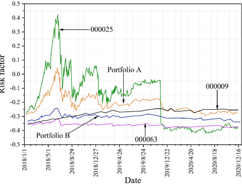
A comparison of the base weight allocation portfolios is shown in Figure 1. The figure visualizes the comparison between the return and volatility between a single fund, Fund Portfolio A and Fund Portfolio B. Since the portfolio consists of five different funds, in order to show the legend more clearly, this paper randomly selects three funds from the constituent funds to compare with the portfolio. Fund codes 000063, 000009 and 000025 are compared with Fund Portfolio A and Fund Portfolio B. It is found that the Fund Portfolio can better iron out the market risk, and the return is more robust under diversification.
In this paper, after using the base weighting scheme portfolios A and B, the base weighting scheme is optimized and managed with the help of Markowitz theory, fuzzy portfolio model, and investor risk characteristics. The management objective is to construct the fund portfolio C so that its risk coefficient is reduced and at the same time its income return is increased.
Based on this, the construction steps of fund portfolio C in this paper are mainly as follows:
(1) Opportunity set stochastic simulation.
(2) Efficient frontier curve generation. In this paper, Monte Carlo simulation experiments are used to simulate the effective frontier curve of Markowitz’s portfolio to obtain the effective frontier curve of the investment effective set in this paper. Using the portfolio model based on fuzzy decision-making to substitute the stochasticity of the securities market with the psychological needs of investors with different risk characteristics, to establish the stochastic fuzzy variables for investors’ risk characteristics.
(3) Fixed risk coefficient. Combined with the risk coefficient of fund portfolio A and fund portfolio B, the risk is weighed in the fund portfolio rationing management, and the fixed risk value in this paper is 0.0715.
| Fund code | Weights of equal weights (fund combination A) | Ratio of risk ratio(fund portfolio B) | Markovitz frontier curve output fund weighting weighting (portfolio C) |
| 000042 | 0.20 | 0.15 | 0.19 |
| 000063 | 0.20 | 0.21 | 0.27 |
| 000012 | 0.20 | 0.16 | 0.05 |
| 000025 | 0.20 | 0.23 | 0.16 |
| 000009 | 0.20 | 0.25 | 0.33 |
| Weight total | 1.00 | 1.00 | 1.00 |
| Standard deviation | 0.1236 | 0.0519 | 0.0715 |
| The yield mean of the scheme | 0.3307 | 0.1267 | 0.3912 |
The weighted rationing optimization scheme is shown in Table 7, and the mean value of the risk coefficient of fund portfolio C is 0.3912.
This paper uses historical data from January 1, 2018 – January 1, 2021 to construct the Fund Portfolio C used in this paper based on Markowitz Portfolio Theory.In this section, this paper will use the data from January 2, 2021 – December 4, 2023 into the historical backtesting of Fund Portfolio C. The data will be used to compare the returns of Fund Portfolio A, Fund Portfolio B, Fund Portfolio C, and two randomly selected funds of different asset classes.
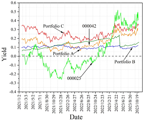
In this summary, the paper compares the simple mean and volatility of returns for Fund Portfolio A, Fund Portfolio B, Fund Portfolio C, and two randomly selected funds of different asset classes using a simple line graph. From the mean and variance of simple returns, from January 2, 2021 – December 4, 2023, Fund Portfolio C has the highest average return. It is about 0.154 units higher than the return of Fund Portfolio A and 0.173 units higher than the return of Fund Portfolio B.
At the same time Fund Portfolio C’s risk remains between Fund Portfolio A and Fund Portfolio B. As a result, the risk-return trade-off of Fund Portfolio C remains valid in the capital market in the first half of 2021-2023. In order to more visually demonstrate the excellent characteristics of Fund Portfolio C, this paper plots a comparison between Fund Portfolio C and two other fund portfolios as well as a randomly selected single fund representing a different broad asset class. The comparison of weighting schemes is shown in Figure 2. A comparison between the three fund portfolios’ returns and volatilities and a typical single fund is shown. In this paper, one bond fund and one equity fund from the underlying assets are randomly selected and the time series of their returns are used to compare the good characteristics of Fund Portfolio C. Taken as a whole, either portfolio effectively irons out market risk. Taken as a whole, Fund Portfolio C belongs to the optimal investment strategy among them. That is, the stochastic portfolio model based on the stochasticity of the securities market with consideration of investors’ risk characteristics has the optimal benefit.
In this paper, we use the fuzzy decision portfolio model to establish a portfolio model based on the stochastic nature of the securities market and the investment behavior of investors considering different risk preference characteristics by considering the return on assets as a random fuzzy variable.
The portfolio benefits under different emotional states or different risk preferences are discussed in separate cases. Taking the meso-emotional state as an example, the trend of the investment ratio of investors under the three risk preferences of risk-averse investors, risk-neutral investors, and risk-seeking investors is consistent. Portfolio benefit and risk are inversely proportional to the sensitivity of risk, the more sensitive investors are to risk, that is, the more risk-averse risk appetite. And as in the case of a certain economic cycle, investor optimism and pessimism will affect the portfolio model.
Optimize the fund portfolio classification allocation with sample MNCs and propose a fuzzy portfolio based fund portfolio C. Comparing the mean and volatility of the returns of different fund portfolios A, B, and C, the stochastic fuzzy return based on investor’s risk characteristics proposed in this paper (fund portfolio C) is higher than that of fund portfolios A and B. When the market is in a state of high volatility, the returns of Fund Portfolio A and Fund Portfolio B will be flat, but the return of Fund Portfolio C can always be maintained at a high level. When the market is at a low level, Fund Portfolio C can effectively stabilize investors’ investment returns and can achieve a higher level of return compared to equity funds.