
Meteorological data are of vital importance to our understanding and prediction of weather and climate, as well as to our response to various weather-related activities. With the continuous development of science and technology, the sources of meteorological data are becoming more and more diversified, including satellites, radars, ground observatories, sounders, etc. [9,15,4,19]. However, these different sources of data often have different characteristics and accuracy, in order to understand the meteorological situation more comprehensively and accurately, meteorological data fusion technology has emerged. Meteorological data fusion is a method of comprehensive processing and analysis of meteorological information from multiple data sources [1,21,13,7]. Its purpose is to integrate data from different sources to obtain more complete, more accurate and more representative meteorological information. The realization of this technique is not simply adding or averaging the data, but needs to take into account the quality of the data, spatial and temporal resolution, error characteristics and other factors [14,6,22,10].
Meteorological radar is a major tool used to monitor rainfall and meteorological phenomena. By observing the radar images, the rainfall situation in each area can be obtained, and the future meteorological trends can also be analyzed to provide basic data for weather forecasting [17,3,18,8]. The working principle of meteorological radar is to utilize the scattering and reflection of RF signals, and by calculating the time, frequency, and phase of the RF signals, we can obtain the reflected signal strength and morphological information of each location in the sky [5,16,20,24]. By processing and analyzing the data from multiple radars, more accurate rainfall and weather trend prediction results can be obtained. The application of weather radar data is very wide. At present, weather radar data have been widely used in weather forecasting, hydrological forecasting, transportation, aerospace, agricultural production and other fields [11,12,23,2].
In this context, the research attempts to innovatively optimize data sources through data fusion based on cloud radar data. Then, combining BP neural network for high-quality analysis of meteorological conditions, it is expected to provide certain technical support for the meteorological industry.
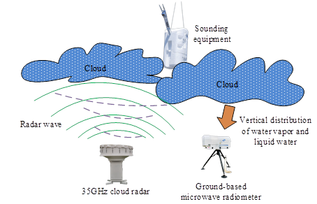
Accurate meteorological forecasting relies on precise monitoring of the weather system, where key data collection can help meteorological professionals predict weather trends. However, meteorological phenomena vary greatly at different time and spatial scales, making high-resolution monitoring difficult. Moreover, there are differences in accuracy and types of data collected by different data collection methods. Cloud radar can obtain detailed information about clouds by emitting radar waves and receiving signals reflected back from water droplets or ice crystals in the cloud layer. Cloud radar is one of the core data sources used to construct data collection methods for meteorological analysis technology. In order to collect more comprehensive meteorological parameters as much as possible, a comprehensive collection system for meteorological analysis data is established based on cloud radar, as shown in Figure 1.
As shown in Figure 1, the comprehensive acquisition system established in the study includes a 35GHz cloud radar, ground-based microwave radiometer, and sounding equipment. The cloud radar emits radar waves and receives signals reflected back from water droplets or ice crystals in the cloud layer, obtaining the vertical structure of the cloud and tracking its development process in real time. Based on the vertical profile information provided by cloud radar, ground-based microwave radiometers detect the vertical distribution of water vapor and liquid water in the atmosphere, while sounding equipment calibrates the data from cloud radar and microwave radiometers. The microwave radiometer provides continuous time series data, filling the gap between each launch of the sounding equipment. However, the data collection equipment itself has noise, and there may also be animals and suspended solids in the detected area, which may affect the quality of the data and require data quality control. This study uses computers to classify reflectance factor data in order to eliminate invalid data. The texture representation of echo intensity is shown in Eq. (1);
\[\label{GrindEQ__1_} IT_{i,j} =\sum _{i=1}^{N}\sum _{j=1}^{N}\left(R_{i,j} -VPR_{i} \right) . \tag{1}\]
In Eq. (1), \(IT_{i,j}\) represents the echo intensity texture at time \(i\) and height \(i\), \(R_{i,j}\) represents the reflectivity factor at time \(i\) and height \(j\) and \(VPR_{i}\) represents the average profile of the reflectance factor in the time direction. The vertical variation of echo intensity is shown in Eq. (2); \[\label{GrindEQ__2_} IG_{i,j} =\sum _{i=1}^{N}\sum _{j=1}^{N}\left(R_{i,j} -VPR_{j} \right) . \tag{2}\]
In Eq. (2), \(IG_{i,j}\) represents the change in echo intensity at time \(i\) and height \(j\). \(VPR_{j}\) represents the average profile of reflectance factors in the vertical direction. According to the analysis results of statistical features, data points are removed when their noise characteristics exceed the preset threshold. The median filtering method is used to further smooth the classified and preliminarily removed reflectance factor data. The median filtering calculation is shown in Eq. (3); \[\label{GrindEQ__3_} R_{filtered} \left(x,y\right)=median\left\{R(x+i,y+j)\right\} . \tag{3}\]
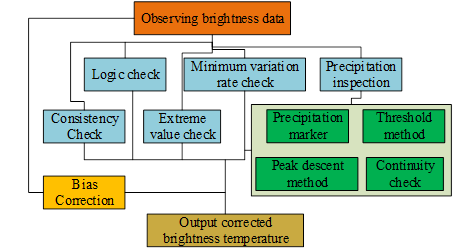
In Eq. (3), \(R_{filtered} \left(x,y\right)\) represents the median filtering result value and \(\left(x,y\right)\) represents the median filtering window. In addition, it is necessary to carry out quality control on the brightness temperature data, which involves a lot of basic information. A quality control system for brightness temperature data is constructed, as shown in Figure 2.
As shown in Figure 2, when controlling the quality of brightness temperature data, it is necessary to combine logical checks, minimum variability checks, precipitation checks, time consistency checks, and extreme value checks. After each inspection, the data will be assigned a corresponding quality identification code, indicating the quality status of the data. If any issues are detected at any step, the data will be marked and enter the error correction process for further correction and processing. Finally, the revised data is generated and a brightness temperature quality label is generated to ensure that the data quality meets the standard. The time consistency check requires calculating the standard deviation of meteorological elements, as shown in Eq. (4);
\[\label{GrindEQ__4_} \sigma =\sqrt{\frac{1}{n} \sum _{i=1}^{n}\left(dE_{t} -d\bar{E}\right)^{2} } . \tag{4}\]
In Eq. (4), \(\sigma\) represents the standard deviation of meteorological elements and \(E_{t}\) represents the meteorological element values at time \(t\) in the time series. After obtaining meteorological data of sufficient quality, subsequent meteorological analysis can begin.
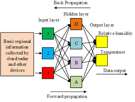
The atmosphere is a complex nonlinear system. The interactions between its various components cannot be simply described by linear models, making the construction and optimization of meteorological prediction models very complex. Moreover, meteorological models usually require a large amount of computing resources and have very high demands on computing power. Data fusion can improve the reliability of overall observations by combining multiple sources of data for mutual verification and correction. BP neural network can effectively capture complex nonlinear relationships between different variables, and automatically optimize their weights through training data to improve data processing efficiency and capability. On the basis of computer data fusion, a meteorological analysis method incorporating BP neural network is proposed. Before conducting meteorological analysis, it is necessary to determine the conditions for judging meteorological conditions. The relative threshold of 85% humidity is set as the boundary. Areas above the boundary are considered to have cloud cover, while areas below the boundary are considered to have no cloud cover. The BP neural network structure for meteorological analysis based on data fusion is shown in Figure 3.
As shown in Figure 3, the data input end of the network receives regional basic information collected by cloud radar and other devices. The data output terminal only sets two sets of data, relative humidity and temperature. The hidden layer is set based on the requirements of the analysis scenario, and the number of layers is determined by repeatedly combining data. Due to the fact that temperature data and humidity data belong to different categories of information, the analysis process of the two types of data is independent of each other. The number of input nodes for the temperature data section is the sum of ground temperature and humidity pressure nodes, channel brightness temperature data nodes, and cloud information nodes. The number of input nodes for the humidity data section is the number of profile layers. The number of hidden layer nodes is estimated using an empirical formula, as shown in Eq. (5):
\[\label{GrindEQ__5_} n_{y} =\sqrt{0.42ab+0.12b^{2} +2.54a+0.77b+0.35} +0.51 . \tag{5}\]
In Eq. (5), \(n_{y}\) represents the number of hidden layer nodes, \(a\) represents the number of nodes in the input layer and \(b\) represents the number of nodes in the output layer. When transferring data between the input layer and the hidden layer, the function calculation is shown in Eq. (6): \[\label{GrindEQ__6_} \tan sig\left(n\right)=\frac{2}{1+e^{-2n} } -1 . \tag{6}\]
In Eq. (6), \(\tan sig\left(n\right)\) represents the tan-Sigmoid function and \(e\) represents the Napier constant. The neural relationship between the hidden layer and the input layer is shown in Eq. (7): \[\label{GrindEQ__7_} Y_{b} =\tan sig\sum _{a=1}^{L}w_{ab} X_{a} +B_{b} . \tag{7}\]
In Eq. (7), \(Y_{b}\) represents the hidden layer neurons, \(X_{a}\) represents input layer neurons, \(w\) represents the weight between two neurons and \(B_{b}\) represents the bias of hidden layer neurons. The neural relationship between the output layer and the hidden layer is shown in Eq. (8): \[\label{GrindEQ__8_} Z_{c} =\sum _{i=1}^{M}w_{bc} Y_{b} +B_{c} . \tag{8}\]
In Eq. (8), \(Z_{c}\) represents the output layer neuron and \(B_{c}\) represents the deviation of output layer neurons. The forward information transmission calculation is shown in Eq. (9): \[\label{GrindEQ__9_} int_{m} =\sum _{i=1}^{n}v_{im} x_{i} . \tag{9}\]
In Eq. (9), \(v_{im}\) represents the input layer information and \(int_{m}\) represents the information transmission from the input layer to the output layer. In information backpropagation, weight adjustment is performed by solving partial derivatives. The forward propagation root mean square error is expanded, as shown in Eq. (10): \[\label{GrindEQ__10_} E_{z} =\frac{1}{2} \sum _{n=1}^{1}\left\{\left[y_{n} -f_{2} \left(\sum _{n=1}^{n}w_{im} Z_{m} \right)\right]\right\} ^{2} . \tag{10}\]
In Eq. (10), \(w_{im}\) represents the intermediate layer information in backpropagation, \(Z_{m}\) represents the last layer of information, \(E_{z}\) represents the forward propagation root mean square error and \(y_{n}\) represents the true output value of the last layer. In order to smoothly operate the meteorological analysis technology designed for research, the constructed computer model framework includes a data collection module, a data preprocessing module, a feature engineering module, a model selection and training module, a model evaluation and validation module, a visualization and result analysis module, and a deployment and monitoring module. Data collection is the starting point of the entire process, determining the quality of the foundational data for subsequent analysis. Data preprocessing and feature engineering ensure that the model is trained using clean and useful data to improve its accuracy. Model training and evaluation are the core components, ensuring the effectiveness of the selected model through scientific selection and evaluation. After completing the model training, the corresponding meteorological conditions can be obtained through information inversion analysis, as shown in Figure 4.
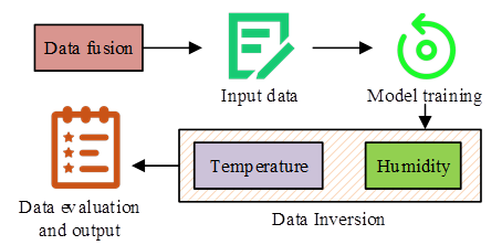
As shown in Figure 4, when conducting specific meteorological condition information inversion, the inversion model data that has undergone data fusion is first input. The BP neural network is trained to establish a mapping relationship from brightness temperature data to temperature and humidity profiles. In the inversion stage, the trained BP neural network inputs real-time observation data into the model. The model predicts temperature and relative humidity profiles based on these data. By comparing with actual sounding data, the effectiveness of the inversion results is evaluated. The optimized parameter details are used as the final meteorological analysis technique to analyze the input data for meteorological analysis.
In order to analyze the operational performance of the meteorological analysis technology designed for research, data availability and computation time are used as testing indicators. During testing, the fused data is input into the computer for processing and corresponding data information is collected. The basic software and hardware environment of the experimental equipment used is shown in Table 1.
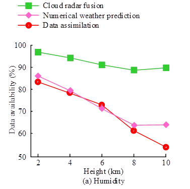
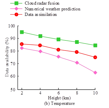
When conducting analysis, the research method is referred to as cloud radar fusion technology. It is compared with current mainstream numerical weather prediction and data assimilation techniques. The collected data was tested for availability, as shown in Figure 5.
As shown in Figure 5, the data availability rate of different methods on different categories of data showed a decreasing trend with increasing height. In Figure 5a, in terms of humidity, the data availability rate of numerical weather prediction was 87.2% at an altitude of 2km, and decreased to 64.9% when the altitude rose to 10km. The data availability of cloud radar fusion technology was 97.3% at an altitude of 2km, and remained above 89.0% at an altitude of 10km. As shown in Figure 5b, in terms of temperature, the data assimilation technique decreased to 77.1% when the altitude increased to 10km. The data availability of cloud radar fusion technology was 95.4% at an altitude of 2km, and remained above 85.0% at an altitude of 10km. The research method can ensure higher data availability and reduce meaningless waste of equipment resources. The calculation time of meteorological analysis results using different methods is analyzed, as shown in Figure 6.
| Parameter variables | Parameter selection |
| Operating system | Windows10 |
| System running memory | 32GB |
| CPU main frequency | 3.30GHz |
| Solid state drive space | 4TB |
| CPU | Intel Core i5-13490 |
| Graphics card model | NVIDIA GeForce Titan X |
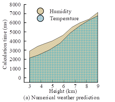
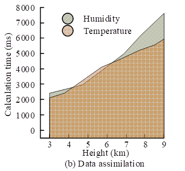
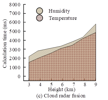
As shown in Figure 6, the computation time of different methods increased with height. In Figure 6a, the calculation time for humidity data in numerical weather prediction reached over 7000ms when the altitude reached 9km. As shown in Figure 6b, the data assimilation technique took more time to calculate temperature data than humidity data when the altitude was between 4km and 7km. The humidity calculation time reached over 7000ms when the altitude reached 9km. As shown in Figure 6c, the cloud radar fusion technology maintained humidity calculation time below 6000ms and temperature calculation time below 5000ms at an altitude of 9km. This indicates that the research method as faster data analysis capability.
In order to analyze the practical application effect of the research method, the research method is used for actual meteorological analysis in the range of Taiyuan ground based remote sensing vertical observation system. The root mean square error is used to analyze the accuracy of the measured relative humidity and temperature profiles. The accuracy of the relative humidity profile is shown in Figure 7.
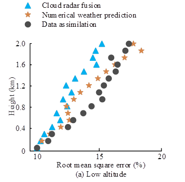
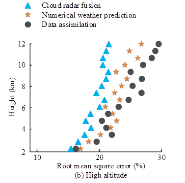
As shown in Figure 7, the root mean square error of the relative humidity profile analyzed by different methods increased with height. In Figure 7a, in low altitude, the root mean square error of the relative humidity profile in the numerical weather prediction reached over 18.0% as the altitude increased to 2km. When the height of cloud radar fusion technology increased to 2km, the root mean square error of the relative humidity profile was 15.4%, with significant fluctuations during the increase process. As shown in Figure 7b, at high altitudes, the root mean square error of the relative humidity profile in numerical weather prediction reached over 27.0% as the altitude increased to 12km. There was a significant pullback during the increase process, but it did not affect the overall trend. When the height increased to 12km, the root mean square error of the relative humidity profile reached over 29.0% in data assimilation technology. The cloud radar fusion technology achieved a root mean square error of 22.0% for the relative humidity profile when the height increased to 12km. However, when the height increased to 7km, the root mean square error of the relative humidity profile no longer showed a significant increasing trend. The accuracy of the temperature profile is shown in Figure 8.
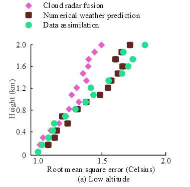
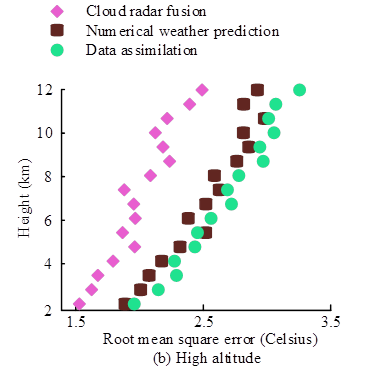
As shown in Figure 8, the root mean square error of the temperature profile analyzed by different method also increased with height. In Figure 8a, in low altitude, the root mean square error of the temperature profile reached over 1.9\(\mathtt{{}^\circ\!{C}}\) when the data assimilation technique increased to an altitude of 2km. When the height increased to 2km, the root mean square error of the temperature profile in cloud radar fusion technology reached 1.5\(\mathtt{{}^\circ\!{C}}\). As shown in Figure 8b, at high altitudes, the root mean square error of the temperature profile in numerical weather prediction reached over 3.0\(\mathtt{{}^\circ\!{C}}\) as the altitude increased to 12km. When the height increased to 12km, the root mean square error of the temperature profile reached over 3.3\(\mathtt{{}^\circ\!{C}}\) using data assimilation technology. When the height increased to 12km, the root mean square error of the temperature profile remained within 2.5\(\mathtt{{}^\circ\!{C}}\) using cloud radar fusion technology. This indicates that the research method has better accuracy in meteorological analysis. The analyzed data is imported into ground based remote sensing vertical observation system to observe the effect, as shown in Figure 9.
As shown in Figure 9, after importing the meteorological analysis results into the urban observation platform, visualized images of temperature profile, relative humidity profile, and cloud particle radii were successfully generated. The temperature profile includes the pressure and temperature conditions corresponding to different time points and heights. The relative humidity profile includes the pressure and relative humidity conditions corresponding to different time points and heights. The cloud particle radius graph displays the variation of cloud particle radius at different time points and heights. Other comprehensive performances are analyzed, as shown in Table 2.
| Indicator | Cloud radar fusion | Numerical weather prediction | Data assimilation |
| Prediction Accuracy (%) | 95.0 | 85.0 | 82.0 |
| Model Convergence Speed (iterations) | 100 | 150 | 130 |
| Resource Utilization (%) | 90.0 | 80.0 | 85.0 |
| Data Redundancy Rate (%) | 5.0 | 10.0 | 8.0 |
| Data Processing Throughput (GB/s) | 4.5 | 3.0 | 3.5 |
| Memory Usage (%) | 70.0 | 85.0 | 80.0 |
As shown in Table 2, among other comprehensive performance metrics, the cloud radar fusion technology had the fastest convergence speed, requiring only 100 iterations. The numerical weather prediction and data assimilation techniques required 150 and 130 iterations, respectively. The resource utilization rate of cloud radar fusion technology reached 90%, which was more efficient in utilizing hardware resources compared with the other two methods. The data processing throughput of cloud radar fusion technology reached 4.5GB/s, higher than the 3.0GB/s of numerical weather prediction and the 3.5GB/s of data assimilation technology, indicating that it could process large amounts of meteorological data more quickly. This indicates that the research method has better operational effectiveness and meteorological analysis accuracy in practical applications.
A meteorological analysis technique combining computer data fusion methods was developed for more accurate meteorological observations. A comprehensive collection system for meteorological analysis data was established based on cloud radar, generating revised data and producing brightness temperature quality indicators to ensure the data quality. A BP neural network structure was constructed for meteorological analysis based on data fusion, and corresponding meteorological conditions were obtained through information inversion analysis. The experimental results showed that when analyzing the calculation time of meteorological analysis results, the research method maintained the humidity calculation time below 6000ms and the temperature calculation time below 5000ms at an altitude of 9km. When conducting accuracy analysis of the results, the research method kept the root mean square error of the temperature profile within 2.5\(\mathtt{{}^\circ\!{C}}\) when the height increased to 12km. The data processing throughput of the research method reached 4.5GB/s, which was higher than other methods. This indicates that the research method has stronger operational efficiency and higher accuracy in conducting meteorological analysis. However, the study does not consider the distortion of meteorological data caused by sudden natural disasters. More sudden parameters will be added to optimize the method in the future to expand the applicability of the research method.
This work was supported by Shanxi Province Meteorological Surface Project: Research on cloud physics feature inversion in Shanxi Province based on cloud radar (SXKMSDW20246752).
The authors declare that they have no conflicts of interest.